Intro
to Ratings.xls
Given a small number of
alternatives, the spreadsheet Ratings.xls helps decision makers select the best
alternative. For example,
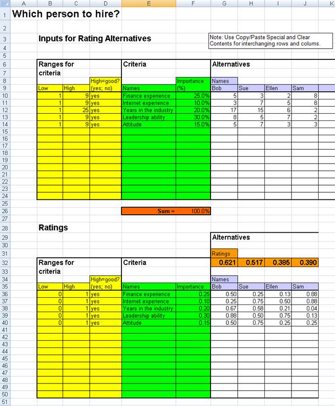
Which
job candidate to hire?
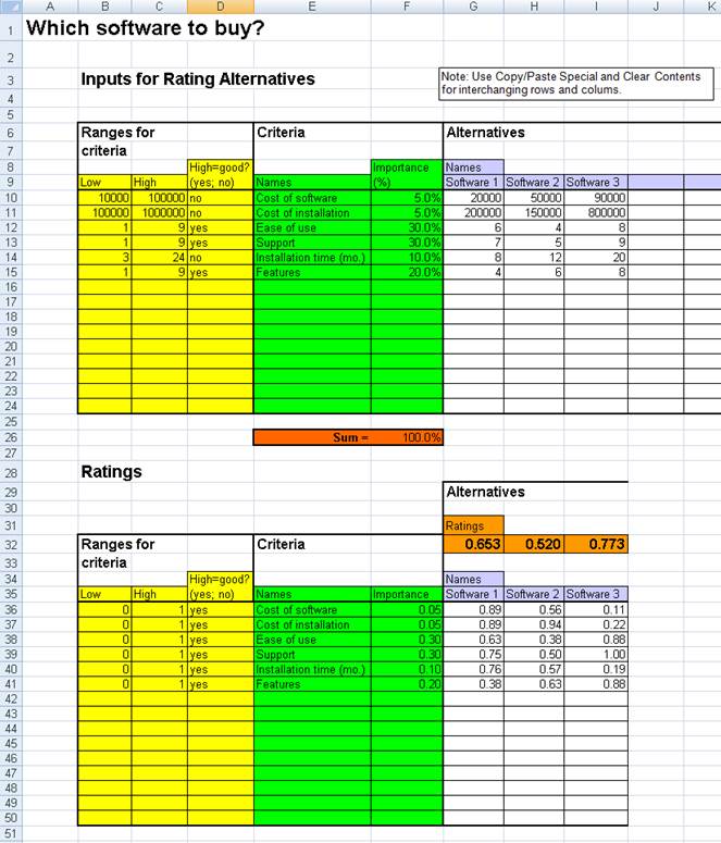
Which
software package to buy?
Which
location to select for a new store or factory?
Which
job to take?
In a
nutshell, here is how Ratings.xls
works. To begin, you enter the alternatives you are considering. (E.g., job
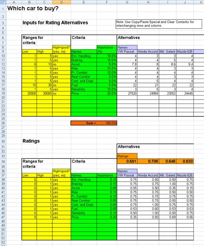
candidates 1,2,3,4.) Next, you enter the criteria that
distinguish the alternatives and the relative importance of these criteria. (E.g.,
years experience (40%), quality of education (40%),
interview performance (20%).) Finally, you enter measures of each alternative
on each criterion within a specified range of values. The spreadsheet then
computes a rating for each alternative; the one with the highest rating is your
best choice. The model is simple in principle, but there are some subtleties. (See
some examples below followed by instructions for using the spreadsheet. See the
spreadsheet for the formulas used.)
You can download Ratings.xls here.
Author:
Mendoza College of Business
University of Notre Dame
Copyright 2016 David Hartvigsen
Examples:
How
to use Ratings.xls
Look at the Input sheet:
1. Enter the names of the
alternatives you are considering.
2. Enter the names of your
criteria for rating the alternatives. This list should address all your
concerns (completeness), but be as short as possible (nonredundancy).
3. In Step 5
you are going to rate, for each criterion, all the alternatives (on
quantitative scales). Before doing this, enter the possible range of ratings
for each criterion. Choose the tightest range that would include ratings of all
alternatives you might reasonably consider (including, of course, the ones you
are considering at present). Specify if the high end of this range corresponds
to a good rating. If a criterion is subjective, then you may specify any range
you like (0 to 100 and 1 to 9 are commonly used).
4. For each criterion enter a
percentage representing the importance of the criterion (considering the range
specified) to your decision; the higher the
percentage, the more important the criterion. Do this so that the sum of the
percentages is 100%. A criterion at 60% should be interpreted
as being three times as important as a criterion at 20%.
5. For each criterion, enter a
rating for each alternative. Make sure that your ratings fall within the ranges
you have set. Note: Suppose Criterion 1 is subjective on a 1 to 9 scale (where
high is better than low). Then a rating of 9 should correspond to the best
possible rating of an alternative you might reasonably consider and a rating of
1 should correspond to the worst possible rating of an alternative you might
reasonably consider (although such alternatives need not be among those
presently being considered). Also, giving Alternative 1 a weight of 6 and
Alternative 2 a weight of 2 means you consider Alternative 1 to be three times
as good as Alternative 2 with respect to this criterion.
Look at the Ratings sheet:
The
highest rating indicates your preferred choice. Note that all the input numbers
have been converted, for consistency, to numbers between 0
and 1; also note that 1 is now the best possible rating for each criterion.
Editing:
Move and delete entries on
the Input sheet using the
Copy/Paste Special/Values and
Clear Contents commands (otherwise the cell references or formatting will get messed up).
Insert additional rows and
columns using the Insert/Rows and Insert/Columns commands. You have to do this
on all worksheets. When not on the Inputs worksheet, you have to use Copy/Paste
Special/Formulas to get the formulas into the new cells.
Delete rows and columns using
the Delete command, as usual.