Geometry of Curves
Nancy K. Stanton
based on original versions © 2000-2005 by Paul Green and Jonathan Rosenberg, modified with permission
Contents
In this published M-file, we will use MATLAB to perform computations and obtain plots involving parametrized curves in two and three dimensions.
Plane Curves
We begin by considering the cycloid, which you have already seen in section 11.1 of Stewart. It is parametrized by (t - sin(t), 1 - cos(t)). We enter the cycloid in MATLAB as a three dimensional curve in order to be able to use the cross-product later on.
syms t
cycloid=[t-sin(t),1-cos(t),0]
cycloid =

[ t - sin(t), 1 - cos(t), 0]
We compute the velocity and acceleration (i.e., the first two derivatives), the speed and the curvature for the cycloid. We will differentiate symbolically with respect to t; however, we do not need to specify t as an argument to diff because MATLAB will automatically differentiate with respect to the variable nearest to x alphabetically, and there is only one variable in this case. First we define a function veclength for computing Euclidean lengths of vectors. We don't want to call it length or norm since those names are already reserved by MATLAB for other purposes.
realdot = @(u, v) u*transpose(v)
veclength = @(v) sqrt(realdot(v,v))
realdot =

    @(u,v)u*transpose(v)


veclength =

    @(v)sqrt(realdot(v,v))
First we compute the velocity, acceleration, and speed:
cycvel = diff(cycloid)
cycacc = diff(cycvel)
cycspeed = simplify(veclength(cycvel))
cycvel =

[ 1 - cos(t), sin(t), 0]


cycacc =

[ sin(t), cos(t), 0]


cycspeed =

2^(1/2)*(1 - cos(t))^(1/2)
From all this we can compute the curvature:
cyccurve = veclength(cross(cycvel,cycacc))/cycspeed^3
cyccurve =

(2^(1/2)*((sin(t)^2 + cos(t)*(cos(t) - 1))^2)^(1/2))/(4*(1 - cos(t))^(3/2))
We can use the pretty command to improve the appearance and intelligibility of the formula for the curvature.
pretty(cyccurve)
   1/2         2                       2 1/2
  2    ((sin(t)  + cos(t) (cos(t) - 1)) )
  ------------------------------------------
                             3
                             -
                             2
               4 (1 - cos(t))
Note that the numerator contains a square followed by a square root, in other words an absolute value. We can get things into better form using simplify. In this example, it works better to simplify the square of the curvature, then take the square root.
cyccurve=sqrt(simplify(cyccurve^2))
cyccurve =

(-1/(8*(cos(t) - 1)))^(1/2)
so
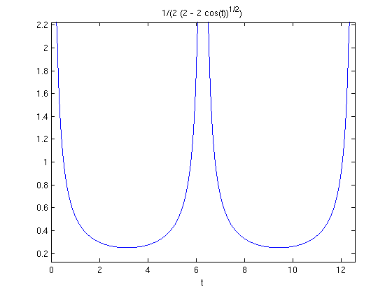
cyccurve=(1/2)/(2-2*cos(t))^(1/2)
cyccurve =

1/(2*(2 - 2*cos(t))^(1/2))
Problem 1
Find symbolic expressions for the velocity, speed, acceleration and curvature for the hypocycloid parametrized by:
hypocyc=[2*cos(t)+cos(2*t),2*sin(t)-sin(2*t),0]
hypocyc =

[ cos(2*t) + 2*cos(t), 2*sin(t) - sin(2*t), 0]
We continue our study of the cycloid. We plot it using ezplot, which will plot a parametrized plane curve provided the first two arguments are the coordinate functions. The last argument gives the range of the parameter for the plot. The command axis normal changes ezplot's default scaling, which would have set the scales on the two axes to be equal.
ezplot(cycloid(1),cycloid(2),[0,4*pi]);axis normal

We have shown two arches of the cycloid in order to show the cusp at  . There are two natural questions. One is the length of each arch, and the other is the behavior of the curvature at the cusp. The length of the cycloid can be computed symbolically, by integrating the speed.
cyclength=int(cycspeed,0,2*pi)
cyclength =

8
Now let us look more carefully at the curvature,  which becomes infinite as cos(t) approaches 1. This behaviour is not apparent from the plot, which makes it look as though the curve becomes straight near the cusp. However it does become apparent from a plot of the curvature as a function of t.
ezplot(cyccurve,[0,4*pi])
Space Curves and Frenet Frames
In this section, we will plot curves in 3-dimensional space and compute their unit tangent, normal, binormal and curvature. In order to have a concrete example before us, we consider the twisted cubic, parametrized by:

syms t
twistcube=[t,t^2,t^3]
twistcube =

[ t, t^2, t^3]
It will be convenient to define a MATLAB function unitvec which converts a vector to a unit vector by dividing the vector by its length:
unitvec = @(v) v/veclength(v)
unitvec =

    @(v)v/veclength(v)
The Frenet frame of a curve at a point is a triple of vectors (T, N, B) consisting of the unit tangent vector T at that point, the unit normal N (the unit vector in the direction of the derivative of the unit tangent with respect to arclength), and the unit binormal B = T × N, the cross-product of the unit tangent with the unit normal. We calculate the Frenet frame for the twisted cubic:
tcvel=diff(twistcube)
tctan=simplify(unitvec(tcvel))
tcacc=diff(tcvel)
tcvel =

[ 1, 2*t, 3*t^2]


tctan =

[ 1/(9*t^4 + 4*t^2 + 1)^(1/2), (2*t)/(9*t^4 + 4*t^2 + 1)^(1/2), (3*t^2)/(9*t^4 + 4*t^2 + 1)^(1/2)]


tcacc =

[ 0, 2, 6*t]
Because the acceleration a is not parallel to the unit normal N, but the cross-product v × a of the velocity and the acceleration is parallel to the unit binormal B, it is convenient to compute the unit binormal before the unit normal vector.
tccross=cross(tcvel,tcacc)
tcbin=simplify(unitvec(tccross))
tccross =

[ 6*t^2, (-6)*t, 2]


tcbin =

[ (3*t^2)/(9*t^4 + 9*t^2 + 1)^(1/2), -(3*t)/(9*t^4 + 9*t^2 + 1)^(1/2), 1/(9*t^4 + 9*t^2 + 1)^(1/2)]
Since T is perpendicular to N and B = T × N, the three unit vectors T, N, and B are mutually perpendicular, and it follows that also N = B × T and T = N × B. This gives the fastest way to compute N.
tcnorm = simplify(cross(tcbin, tctan))
tcnorm =

[ -(t*(9*t^2 + 2))/((9*t^4 + 4*t^2 + 1)^(1/2)*(9*t^4 + 9*t^2 + 1)^(1/2)), -(9*t^4 - 1)/((9*t^4 + 4*t^2 + 1)^(1/2)*(9*t^4 + 9*t^2 + 1)^(1/2)), (3*t*(2*t^2 + 1))/((9*t^4 + 4*t^2 + 1)^(1/2)*(9*t^4 + 9*t^2 + 1)^(1/2))]
We recall that the curvature, while defined as the magnitude of the derivative of the unit tangent with respect to arclength, is most conveniently computed as follows:
tccurve=simplify(veclength(tccross)/veclength(tcvel)^3)
tccurve =

(2*(9*t^4 + 9*t^2 + 1)^(1/2))/(9*t^4 + 4*t^2 + 1)^(3/2)
Problem 2
Consider the trefoil parametrized by
trefoil=[(2+cos(3*t))*cos(2*t),(2+cos(3*t))*sin(2*t),cos(3*t)]
trefoil =

[ cos(2*t)*(cos(3*t) + 2), sin(2*t)*(cos(3*t) + 2), cos(3*t)]
- (a) Plot the trefoil for t between 0 and
 .
. - (b) Compute the curvature of the trefoil.
- (c) Compute the Frenet frame of the trefoil.
To view the Frenet frame geometrically, we use the M-file curveframeplot.m. This plots the curve in blue together with normal vectors in red and binormal vectors in green. The tangent vectors are not plotted since the tangent direction is clear from the curve. The last two arguments determine the number of frames plotted and the length of the normal and binormal vectors.
type curveframeplot
% This is an M-file intended to plot a space curve together with
% several instances of the Frenet Frame, represented by the
% normal in red and the unit binormal in green. The
% parameter num determines the number of frames plotted; the
% parameter len determines the length of the frame vectors.

function  z = curveframeplot(curve, parameter, start, fin, num, len)

newcurve=subs(curve, parameter, 't');
t= start:.01*(fin-start):fin;
x = eval(vectorize(newcurve(1)));
y = eval(vectorize(newcurve(2)));
w = eval(vectorize(newcurve(3)));
plot3(x,y,w)
hold on

unitvec = @(u) u/sqrt(u*transpose(u));
curvevel=diff(curve);
curvetan=unitvec(curvevel);
curvenorm=unitvec(diff(curvetan));
curvebin=cross(curvetan,curvenorm);

t1=start:(fin-start)/num:fin;
newcurve1=subs(curve,parameter,'t1');
norm1=subs(curvenorm,parameter,'t1');
bin1=subs(curvebin,parameter,'t1');
x1 = eval(vectorize(newcurve1(1)));
y1 = eval(vectorize(newcurve1(2)));
w1 =eval(vectorize(newcurve1(3)));
xnorm = eval(vectorize(newcurve1(1)+len*norm1(1)));
ynorm = eval(vectorize(newcurve1(2)+len*norm1(2)));
wnorm=eval(vectorize(newcurve1(3)+len*norm1(3)));
xbin = eval(vectorize(newcurve1(1)+len*bin1(1)));
ybin = eval(vectorize(newcurve1(2)+len*bin1(2)));
wbin =eval(vectorize(newcurve1(3)+len*bin1(3)));

for n=1:length(t1)
   plot3([x1(n),xnorm(n)],[y1(n),ynorm(n)],[w1(n),wnorm(n)],'red')
   plot3([x1(n),xbin(n)],[y1(n),ybin(n)],[w1(n),wbin(n)],'green')
end
hold off
curveframeplot(twistcube,'t',-1,1,10,.2)

Notice how the Frenet frames twist around the curve as the parameter changes. To make this even clearer, we define and plot a tube around the curve. We will need a second parameter since the tube is a surface.
syms s
tctube=twistcube+ .2*cos(s)*tcnorm+.2*sin(s)*tcbin ;
pretty(tctube)
  +-                                                                                                                                                                                                                                -+
  |              2                                         2                                                                         4                                                                            2                  |
  |           3 t  sin(s)                     t cos(s) (9 t  + 2)               2         3 t sin(s)                      cos(s) (9 t  - 1)                       sin(s)            3              3 t cos(s) (2 t  + 1)             |
  |  t + ---------------------- - -------------------------------------------, t  - ---------------------- - -------------------------------------------, ---------------------- + t  + -------------------------------------------  |
  |            4      2     1/2         4      2     1/2     4      2     1/2             4      2     1/2         4      2     1/2     4      2     1/2        4      2     1/2              4      2     1/2     4      2     1/2  |
  |      5 (9 t  + 9 t  + 1)      5 (9 t  + 4 t  + 1)    (9 t  + 9 t  + 1)          5 (9 t  + 9 t  + 1)      5 (9 t  + 4 t  + 1)    (9 t  + 9 t  + 1)     5 (9 t  + 9 t  + 1)           5 (9 t  + 4 t  + 1)    (9 t  + 9 t  + 1)     |
  +-                                                                                                                                                                                                                                -+
In this case, the input is more illuminating than the output. For fixed t, s parametrizes a circle around the tube. For fixed s, t parametrizes a curve running along the tube and, in the presence of torsion, twisting around it. We will plot the tube using ezmesh. The first three arguments are the components of tctube; the last argument gives the limits for s and t in the form [smin, smax, tmin, tmax]:
ezmesh(tctube(1),tctube(2),tctube(3),[0,2*pi,-1,1])
title('Tube around a twisted cubic')

Notice the way in which the longitudinal mesh lines, corresponding to constant values of s, twist around the tube.
The twisting is measured by the torsion  which is defined by

If you are interested, you can find more information about torsion in Stewart, section 14.3, exercises #53-55.
Problem 3
- (a) Use curveframeplot to plot the trefoil with its Frenet frame.
- (b) Use ezmesh to show the twisting of the Frenet frame of the trefoil around the curve.
Additional Problems
1) Observe that any curve given in polar coordinates by  can be parametrized as (f(t)cos(t), f(t)sin(t)). Use this observation to analyze each of the following curves. Plot each curve, compute its length (numerically if MATLAB can't do it symbolically), plot the curvature as a function of t, determine the curvature bounds, and identify any cusps or self-intersections. When possible simplify your answer using simplify or simple.
- The cardioid

- The lemniscate

- The limacon

2) Observe that the graph of a function f can be parametrized as (t, f(t)). Use this observation to analyze the graph of each of the following functions. Determine the curvature bounds if they exist, compute the length of each graph between x = 0 and x = 1, and identify any cusps:
- x^2
- x^3
- x^4
- x^(3/2)
- e^x
3) Consider the family of helices parametrized by (R cos(t),R sin(t),A t).
- (a) Compute the curvature as a function of R and A.
- (b) For R = A = 1, plot the helix, showing the Frenet frame at several points along the curve.
- (c) Plot the tube of radius .2 around the helix showing the twisting of the Frenet frame around the helix.