Graphs of the beta density

Here are graphs of the beta density for different values of the parameters. From the graphs you can imagine how changing the parameters would allow you to fit a beta density to a wide variety of data sets. In fact, MATLAB has a command betafit designed to do that.

a=b=1.5
a=b=0.5
a=b=0.75
a=b=2.5
a=0.5, b=2.5
a=2.5, b=0.5
a=0.75, b=0.5
a=b=3.5
a=b=5
a=5, b=3
a=5, b=1.5
a=7, b=2
a=2, b=7.5

I begin by creating a vector of $X$ values to plot, with 1000 equally spaced points in [0,1].

X = linspace(0,1,1000);

The command betapdf(X,a,b) computes the values of the beta density with parameters $a$ and $b$ at the points of $X$ . I'll use that to plot. After each plot I give two commands to change the tick marks on the $x$ axis to go from 0 to 1 instead of 0 to 1000 (the values of $X$ ).

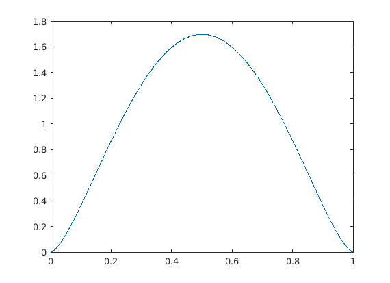
a=b=1.5

plot(betapdf(X,1.5,1.5))
ax=gca;
ax.XTickLabel = {'0','0.2','0.4','0.6','0.8','1'};

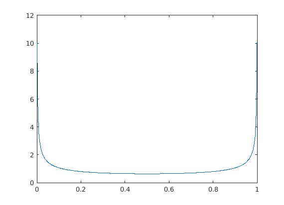
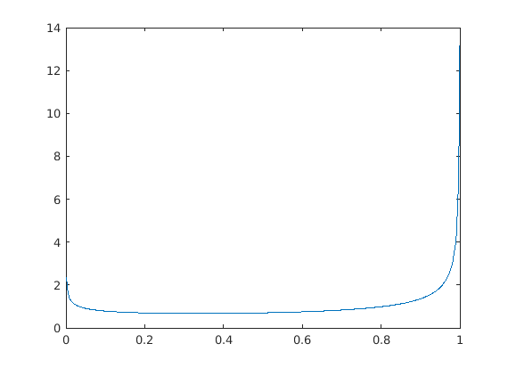
a=b=0.5

plot(betapdf(X,0.5,0.5))
ax=gca;
ax.XTickLabel = {'0','0.2','0.4','0.6','0.8','1'};

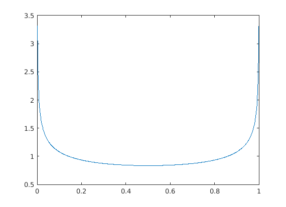
a=b=0.75

plot(betapdf(X,0.75,0.75))
ax=gca;
ax.XTickLabel = {'0','0.2','0.4','0.6','0.8','1'};

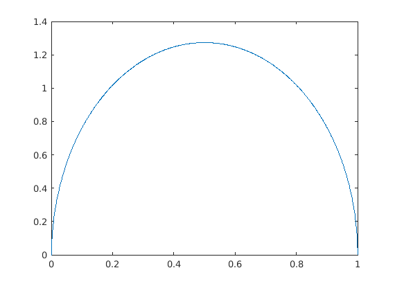
a=b=2.5

plot(betapdf(X,2.5,2.5))
ax=gca;
ax.XTickLabel = {'0','0.2','0.4','0.6','0.8','1'};

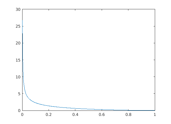
a=0.5, b=2.5

plot(betapdf(X,0.5,2.5))
ax=gca;
ax.XTickLabel = {'0','0.2','0.4','0.6','0.8','1'};

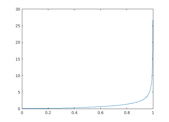
a=2.5, b=0.5

plot(betapdf(X,2.5,0.5))
ax=gca;
ax.XTickLabel = {'0','0.2','0.4','0.6','0.8','1'};

a=0.75, b=0.5

plot(betapdf(X,0.75,0.5))
ax=gca;
ax.XTickLabel = {'0','0.2','0.4','0.6','0.8','1'};

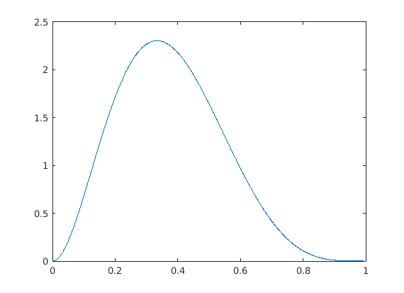
a=b=3.5

plot(betapdf(X,3,5));
ax=gca;
ax.XTickLabel = {'0','0.2','0.4','0.6','0.8','1'};

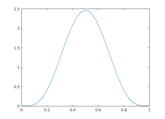
a=b=5

plot(betapdf(X,5,5));
ax=gca;
ax.XTickLabel = {'0','0.2','0.4','0.6','0.8','1'};

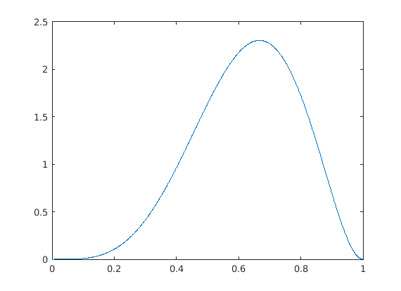
a=5, b=3

plot(betapdf(X,5,3))
ax=gca;
ax.XTickLabel = {'0','0.2','0.4','0.6','0.8','1'};

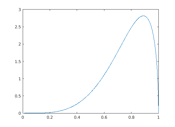
a=5, b=1.5

plot(betapdf(X,5,1.5))
ax=gca;
ax.XTickLabel = {'0','0.2','0.4','0.6','0.8','1'};

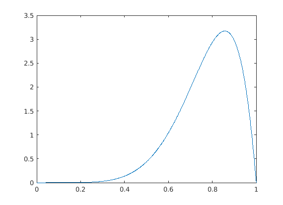
a=7, b=2

plot(betapdf(X,7,2))
ax=gca;
ax.XTickLabel = {'0','0.2','0.4','0.6','0.8','1'};

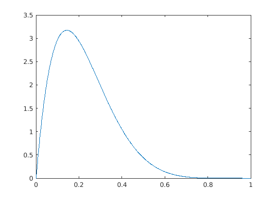
a=2, b=7.5

plot(betapdf(X,2,7))
ax=gca;
ax.XTickLabel = {'0','0.2','0.4','0.6','0.8','1'};