Normal density function
Contents
Plots of the normal density function
The MATLAB function normpdf gives the normal probability density function. If X is a vector then the command normpdf(X,mu,sigma) computes the normal density with parameters mu and sigma at each value of X. The command normpdf(X) computes the standard normal density at each value of X.
X = [-5:0.01:5];
Standard normal density
plot(X,normpdf(X))
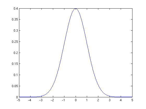
The plot shows a bell shaped curve.
mu=1,sigma=1
plot(X,normpdf(X,1,1))
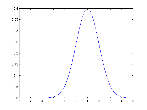
We see the point where the graph peaks has shifted.
mu=0, sigma=2
We plot this in red along with the standard normal in blue.
plot(X,normpdf(X))
hold on
plot(X,normpdf(X,0,2),'Color','r')
hold off
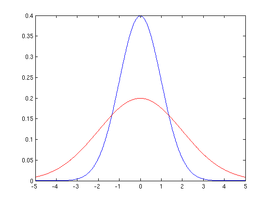
The plot is more spread out and has a lower peak with larger sigma.
mu=0, sigma = 1/2
We plot this in green along with the standard normal in blue
plot(X,normpdf(X))
hold on
plot(X,normpdf(X,0,1/2),'Color','g')
hold off
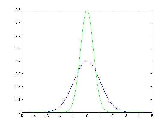
The plot is more concentrated near x=0 and the peak is higher.
Binomial distribution
Here are some plots we looked at when we did the binomial distribution, first with p=1/2, n=100, then with p=1/3, n=100.
binomplot(100,1/2)
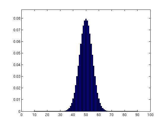
Notice the resemblance to a normal density.
binomplot(100,0.3)
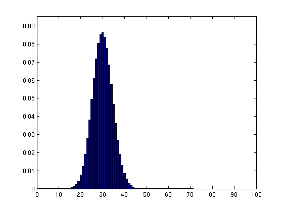
Again, notice the resemblance to a normal density.
Cumulative distribution function
The MATLAB command normcdf(X,mu,sigma) gives the cumulative distribution function of the normal density with parameters mu, sigma. The command normcdf(X) gives the cumulative distribution function of the standard normal density.
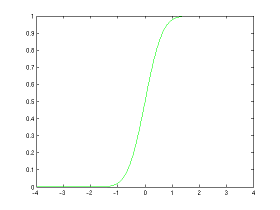
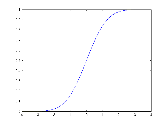
Standard normal cumulative distribution function
X = -4:0.01:4;
plot(X,normcdf(X))
mu=1,sigma=1
plot(X,normcdf(X,1,1))
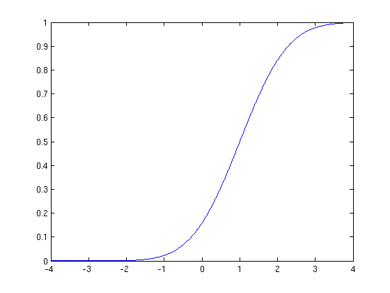
Changing mu translates it.
mu=0, sigma=2
plot(X,normcdf(X,0,2),'Color','r')
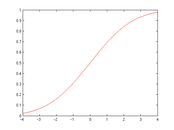
With larger sigma it approaches 1 more slowly.
mu=0, sigma=1/2
plot(X,normcdf(X,0,1/2),'Color','g')
% With smaller sigma it approaches more rapidly.