Section 7.1

Contents

Computing the convolution of two vectors

The MATLAB command conv lets you compute the convolution of two vectors. So, for example, if u, v are given by

u = [1/4 1/4 1/2]
v = [1/9 2/9 1/9 1/3 1/18 1/6]

u =

    0.2500    0.2500    0.5000


v =

    0.1111    0.2222    0.1111    0.3333    0.0556    0.1667

their convolution is

conv(u,v)

ans =

  Columns 1 through 7

    0.0278    0.0833    0.1389    0.2222    0.1528    0.2222    0.0694

  Column 8

    0.0833

Rolling a die 10 times

Suppose you are interested in the distribution that results from rolling a die 10 times. The distribution for rolling once is:

w = [1/6 1/6 1/6 1/6 1/6 1/6]

w =

    0.1667    0.1667    0.1667    0.1667    0.1667    0.1667

The distribution for the sum is the convolution of w with itself 9 times. Here's a way to compute it.

p = w; % initialize p.
for j = 1:9
    p = conv(p,w); % p is the result of convolving w with itself j times
end

The resulting distribution is:

p

p =

  Columns 1 through 7

    0.0000    0.0000    0.0000    0.0000    0.0000    0.0000    0.0001

  Columns 8 through 14

    0.0002    0.0004    0.0008    0.0014    0.0024    0.0040    0.0063

  Columns 15 through 21

    0.0095    0.0137    0.0190    0.0254    0.0326    0.0405    0.0485

  Columns 22 through 28

    0.0561    0.0629    0.0682    0.0715    0.0727    0.0715    0.0682

  Columns 29 through 35

    0.0629    0.0561    0.0485    0.0405    0.0326    0.0254    0.0190

  Columns 36 through 42

    0.0137    0.0095    0.0063    0.0040    0.0024    0.0014    0.0008

  Columns 43 through 49

    0.0004    0.0002    0.0001    0.0000    0.0000    0.0000    0.0000

  Columns 50 through 51

    0.0000    0.0000

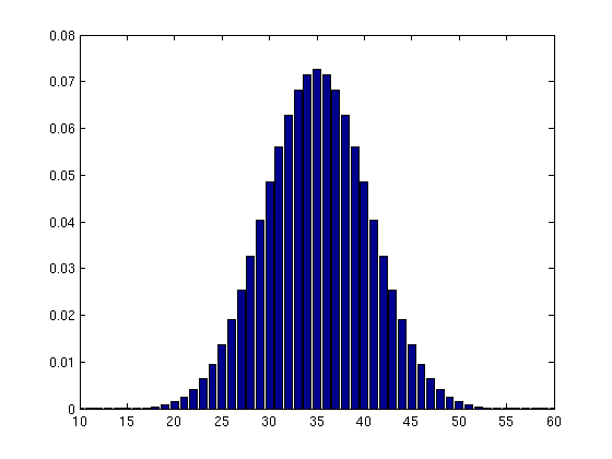
A good way to make sense of this is to view it as a bar graph. Now the values of p range from 10 to 60.

bar(10:60,p)
axis([10 60 0 0.08])

Published with MATLAB® R2014a