SECTION 8.1 - EULER'S METHOD

Here I use the function myeuler (from pages 104-105 of Differential Equations with MATLAB) implementing Euler's method to solve y' = 2y - 1. It takes as input the function f, the inital time tinit, the initial y-value yinit, the final time value b and the number of steps n.

syms t y
f = @(t,y) 2*y - 1

f = 

    @(t,y)2*y-1

First we use step size 0.1.

[t1,y1] = myeuler(f,0,1,0.4,4); [t1,y1]

ans =

         0    1.0000
    0.1000    1.1000
    0.2000    1.2200
    0.3000    1.3640
    0.4000    1.5368

Next we use step size 0.05.

[t2,y2] = myeuler(f,0,1,0.4,8); [t2,y2]

ans =

         0    1.0000
    0.0500    1.0500
    0.1000    1.1050
    0.1500    1.1655
    0.2000    1.2321
    0.2500    1.3053
    0.3000    1.3858
    0.3500    1.4744
    0.4000    1.5718

Finally we use step size 0.025

[t3,y3] = myeuler(f,0,1,0.4,16); [t3,y3]

ans =

         0    1.0000
    0.0250    1.0250
    0.0500    1.0513
    0.0750    1.0788
    0.1000    1.1078
    0.1250    1.1381
    0.1500    1.1700
    0.1750    1.2036
    0.2000    1.2387
    0.2250    1.2757
    0.2500    1.3144
    0.2750    1.3552
    0.3000    1.3979
    0.3250    1.4428
    0.3500    1.4900
    0.3750    1.5395
    0.4000    1.5914

The exact solution is

y = dsolve('Dy = 2*y-1, y(0) = 1','t')

 
y =
 
exp(2*t)/2 + 1/2

Here is a table of values. The first entry is t, followed by the approximate solutions evaluated at that value of t, followed by the exact solution evaluated at that value of t. We build the table T a row at a time using a for loop. We initialize T as an empty matrix.

format short
T = [ ];
for k=0:4
    A = [t1(k+1),y1(k+1),y2(2*k+1),y3(4*k+1),subs(y,'t',t1(k+1))];
    T = [T;A];
end
T

T =

         0    1.0000    1.0000    1.0000    1.0000
    0.1000    1.1000    1.1050    1.1078    1.1107
    0.2000    1.2200    1.2321    1.2387    1.2459
    0.3000    1.3640    1.3858    1.3979    1.4111
    0.4000    1.5368    1.5718    1.5914    1.6128

We plot the three approximate solutions and the exact solution.

plot(t1,y1,'c'), hold on
plot(t2,y2,'r')
plot(t3,y3,'g')
ezplot(y,[0,0.4])
title 'Solutions using Eulers method and the exact solution'
legend1 = legend({'step size 0.1', 'step size 0.05', 'step size 0.025','exact'},'Position',[0.1465 0.7205 0.2171 0.1869]);
hold off

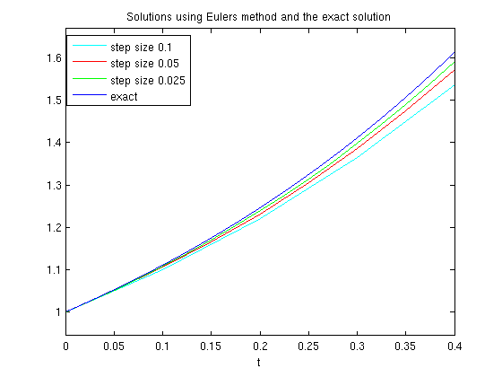
We see from both the plot and the table that the error in the approximate solutions decreases as the number of steps increases, but it is still fairly large.