Section 8.1 - Euler's Method

Why is it often necessary to use graphical and numerical techniques?

Why is it often necessary to use graphical and numerical techniques?

Here is an example of an ODE which MATLAB claims to solve explicitly, but the solution is very complicated. The initial value problem is

$y'=y^2+t^2, \quad y(0)=1.$

Here is MATLAB's "exact solution."

y = dsolve('Dy = y^2 + t^2, y(0)=1', 't'); pretty(y)

Warning: Explicit solution could not be found; implicit solution returned. 
Warning: The solutions are parametrized by the symbols:
z = solve([limit((4*t*gamma(3/4)*besselK(-3/4, (t^2*I)/2)*I -
2^(1/2)*4^(1/4)*C6*PI^(3/2)*t*besselI(-3/4, (t^2*I)/2)*I)/(4*gamma(3/4)*besselK(1/4,
(t^2*I)/2) + 2^(1/2)*4^(1/4)*C6*PI^(3/2)*besselI(1/4, (t^2*I)/2)), t = 0) = 1], C6,
VectorFormat = TRUE)
 

                                        1/2  1/4   3/2
  4 t gamma(3/4) besselk(-3/4, #1) i - 2    4    pi    t z besseli(-3/4, #1) i
  ----------------------------------------------------------------------------
                                        1/2  1/4   3/2
       4 gamma(3/4) besselk(1/4, #1) + 2    4    pi    z besseli(1/4, #1)
  
  where
  
           2
          t  i
     #1 = ----
           2

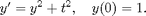
The solution is very complicated and involves $z$ , which is the solution of a very complicated equation. Also, it gives me an absurd plot:

ezplot(y)

There is a discussion of this example and how to solve it using MuPad on pp;. 72-74 of Differential Equations with MATLAB.

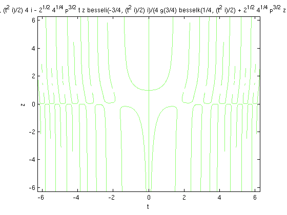
We can solve it exactly using Maple, with the command:

dsolve({diff(y(t), t) = y(t)^2+t^2, y(0) = 1}, y(t))

The solution is:

syms t
y = -t*(-(gamma(3/4)^2-pi)/gamma(3/4)^2*besselj(-3/4,1/2*t^2)+...
    bessely(-3/4,1/2*t^2))/(-(gamma(3/4)^2-pi)/gamma(3/4)^2*besselj(1/4,1/2*t^2)...
    +bessely(1/4,1/2*t^2));

To get a better idea of what the solution is like, we can view it graphically. One method is to plot the solution.

ezplot(y,[0,0.8])
xlabel 't', ylabel 'y'
title 'Solution of dy/dt = y^2 + t^2'

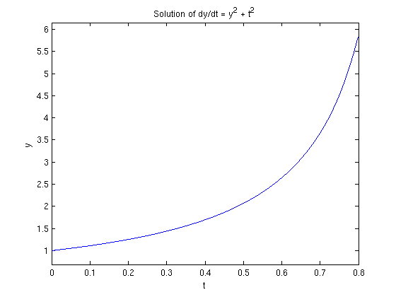
Another method is to look at the direction field using the quiver command.

[T,Y] = meshgrid(-3:0.2:3,-3:0.2:3);
S = T.^2 + Y.^2;
L = sqrt(1 + S.^2);
quiver(T, Y, 1./L, S./L, 0.5), axis tight
xlabel 't', ylabel 'y'
title 'Direction field for dy/dt = y^2 + t^2'

A third method is to solve numerically and plot the resulting numerical solution. Here we do that using ode45.

f = @(t,y) y^2 + t^2;
ode45(f,[0,0.8],1)

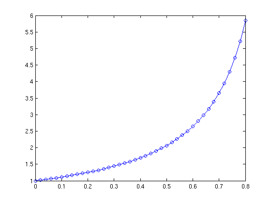
Note that this plot looks the same as what we found when we plotted the explicit solution.

Here's another example where MATLAB finds a very complicated solution.

$y' = y^2 + t, \quad y(0)=0.$

y = dsolve('Dy = y^2 + t, y(0) = 0','t')

 
y =
 
(airyBi(-t, 1) + 3^(1/2)*airyAi(-t, 1))/(airyBi(-t, 0) + 3^(1/2)*airyAi(-t, 0))

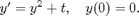
Here's the direction field.

[T,Y] = meshgrid(-3:0.2:3,-3:0.2:3);
S = T + Y.^2;
L = sqrt(1 + S.^2);
quiver(T, Y, 1./L, S./L, 0.5), axis tight
xlabel 't', ylabel 'y'
title 'Direction field for dy/dt = y^2 + t'

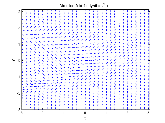
If we attempt to plot the exact solution, we run into a problem. MATLAB doesn't seem to know what airyAi and airyBi are. Here's a way around that. These functions come from MuPad and haven't been converted to MATLAB notation. (This example is discussed on pp. 61-63 of Differential Equations with MATLAB.)

tvals = 0:0.01:2;
plot(tvals,double(subs(y,'t',tvals)))
xlabel 't', ylabel 'y'
title 'Exact solution'

Can this be correct?

Alternatively we can plot the numerical solution obtained with ode45.

f = @(t,y) y^2 + t;
[t,ya] = ode45(f,[0,2],0);
plot(t,ya)

Warning: Failure at t=1.986314e+00.  Unable to meet integration tolerances without
reducing the step size below the smallest value allowed (3.552714e-15) at time t.

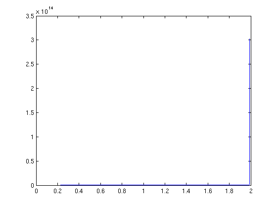
Can this be correct?

Here is a problem MATLAB can't solve exactly.

$y' = \mbox{--}\,t^2 y^3 + \cos(t), \quad y(0) = 0.$

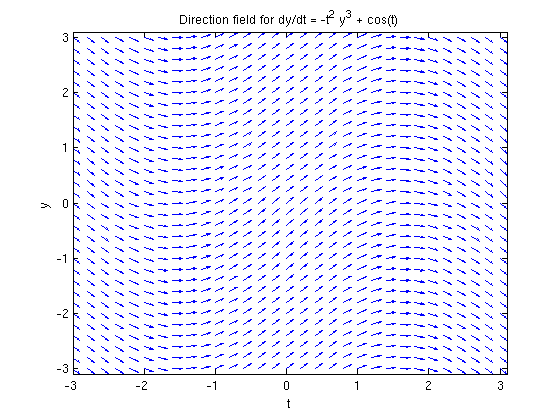
There is no choice but to use graphical and numerical techniques to analyze this equation. Here is the direction field.

[T,Y] = meshgrid(-3:0.2:3,-3:0.2:3);
S = -T.^2*Y.^3  + cos(T);
L = sqrt(1 + S.^2);
quiver(T, Y, 1./L, S./L, 0.5), axis tight
xlabel 't', ylabel 'y'
title 'Direction field for dy/dt = -t^2 y^3 + cos(t)'

Here is a plot of the numerical solution obtained with ode45.

f = @(t,y) -t^2*y^3 + cos(t);
[t,ya] = ode45(f,[0:100],0);
plot(t,ya)

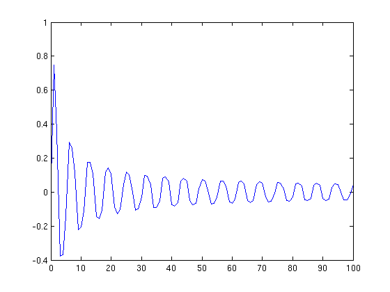
From this we see that the solution appears to tend slowly towards 0 in an oscillating manner as x gets very large.

Section 8.1 - Euler's Method

Contents

Why is it often necessary to use graphical and numerical techniques?