Fourier Series
You can use the following commands to calculate the  partial sum of the Fourier series of the expression
  on the interval
 ![$[-L,L]$](fourier_series2_eq56081.png) .
.
syms x k L n
evalin(symengine,'assume(k,Type::Integer)');
a = @(f,x,k,L) int(f*cos(k*sym('pi')*x/L)/L,x,-L,L);
b = @(f,x,k,L) int(f*sin(k*sym('pi')*x/L)/L,x,-L,L);
fs = @(f,x,n,L) a(f,x,0,L)/2 + ...
    symsum(a(f,x,k,L)*cos(k*pi*x/L) + b(f,x,k,L)*sin(k*pi*x/L),k,1,n);
pfs = @(f,x,n,L) pretty(simple(fs(f,x,n,L)));
I'll do it for the function  on the interval
 ![$[-1,1]$](fourier_series2_eq85290.png) .
.
f =

abs(x)
f = abs(x)
The partial sum is
fs(f,x,n,1)
ans =

1/2 - (2*sum(((exp(-pi*k*x*i)/2 + exp(pi*k*x*i)/2)*(2*((exp(-(pi*k*i)/2)*i)/2 - (exp((pi*k*i)/2)*i)/2)^2 - pi*k*((exp(-pi*k*i)*i)/2 - (exp(pi*k*i)*i)/2)))/k^2, k == 1..n))/pi^2
Here's a more readable form.
pfs(f,x,n,1)
      n
     ---                   k
     \    cos(pi k x) ((-1)  - 1)
  2  /    -----------------------
     ---             2
    k = 1           k
  ------------------------------- + 1/2
                  2
                pi
The Fourier series is
pfs(f,x,inf,1)
           Inf              /      / pi k \2                  \
           ---  cos(pi k x) | 2 sin| ---- |  - pi k sin(pi k) |
           \                \      \  2   /                   /
        2  /    -----------------------------------------------
           ---                         2
          k = 1                       k
  1/2 - -------------------------------------------------------
                                    2
                                  pi
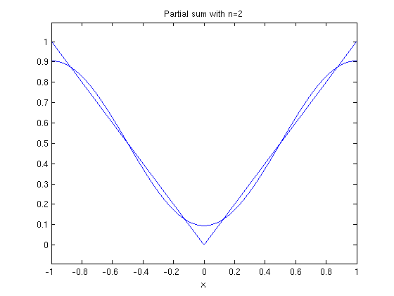
Here are the plots of the partial sums for  . The plot also shows the function .
ezplot(fs(f,x,2,1),-1,1)
hold on
ezplot(f,-1,1)
hold off
title('Partial sum with n=2')
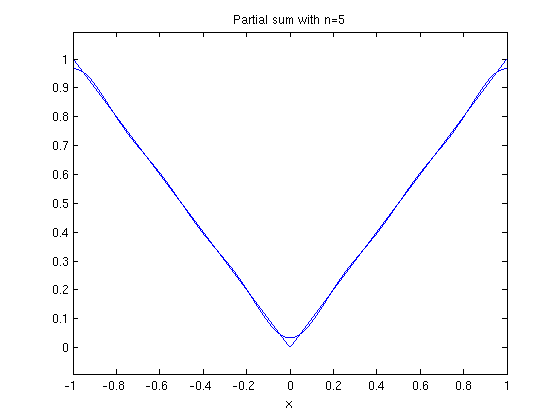
ezplot(fs(f,x,5,1),-1,1)
hold on
ezplot(f,-1,1)
hold off
title('Partial sum with n=5')
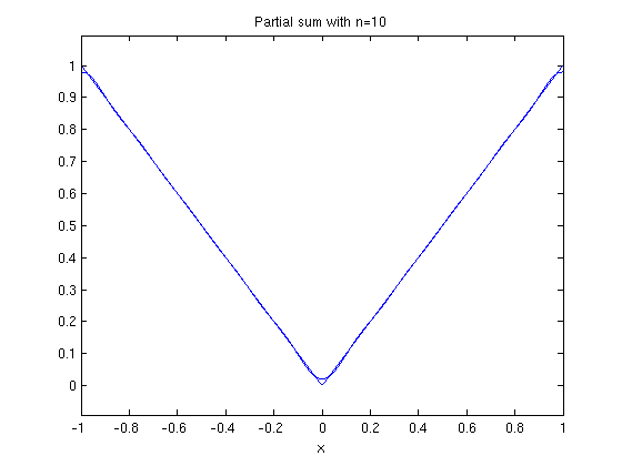
ezplot(fs(f,x,10,1),-1,1)
hold on
ezplot(f,-1,1)
hold off
title('Partial sum with n=10')
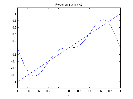
Now I do it with the function  on .
on .
f = x

fs(f,x,n,1)
f =

x


ans =

-(2*sum((((exp(-pi*k*x*i)*i)/2 - (exp(pi*k*x*i)*i)/2)*(- (exp(-pi*k*i)*i)/2 + (exp(pi*k*i)*i)/2 + pi*k*(exp(-pi*k*i)/2 + exp(pi*k*i)/2)))/k^2, k == 1..n))/pi^2
pfs(f,x,n,1)
        n
       ---      k
       \    (-1)  sin(pi k x)
    2  /    -----------------
       ---          k
      k = 1
  - -------------------------
               pi
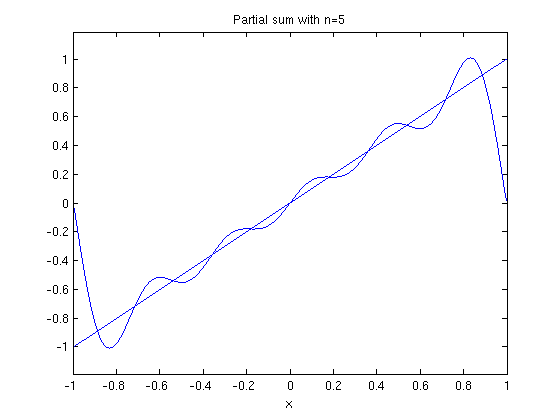
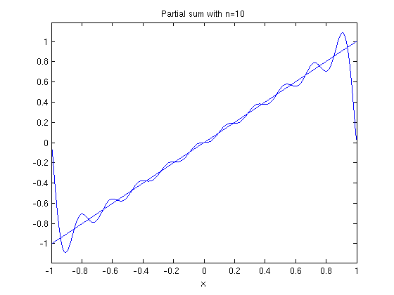
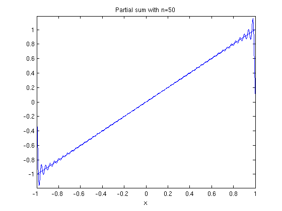
Here are plots of the partial sums for 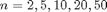 .
.
ezplot(fs(f,x,2,1),-1,1)
hold on
ezplot(f,-1,1)
hold off
title('Partial sum with n=2')
ezplot(fs(f,x,5,1),-1,1)
hold on
ezplot(f,-1,1)
hold off
title('Partial sum with n=5')
ezplot(fs(f,x,10,1),-1,1)
hold on
ezplot(f,-1,1)
hold off
title('Partial sum with n=10')
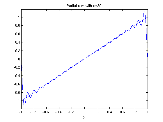
ezplot(fs(f,x,20,1),-1,1)
hold on
ezplot(f,-1,1)
hold off
title('Partial sum with n=20')
ezplot(fs(f,x,50,1),-1,1)
hold on
ezplot(f,-1,1)
hold off
title('Partial sum with n=50')
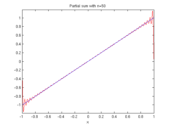
If you zoom in here, you notice that the graph of the partial sum of the Fourier series looks very jagged. That is because ezplot does not plot enough points compared to the number of oscillations in the functions in the partial sum. We can fix this problem using plot. This also allows us to use a different colors for the plot of the original function and the plot of the partial sum. To use plot, we need to turn the partial sum into an inline vectorized function and specify the points where it will be evaluated.
g = inline(vectorize(fs(f,x,50,1)));
X = -1:.001:1;
plot(X,g(X),'r')
hold on
ezplot(f,-1,1)
hold off
title('Partial sum with n=50')
g = inline(vectorize(fs(f,x,100,1)));
X = -1:.0005:1;
plot(X,g(X),'r')
hold on
ezplot(f,-1,1)
hold off
title('Partial sum with n=100')
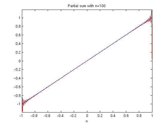
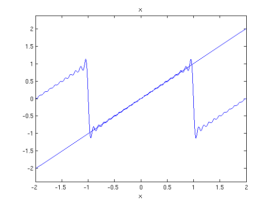
Notice that no matter how many terms we take, the partial sum always overshoots the function  at the end points of the interval. If we do our two plots on the interval
 ![$[-2,2]$](fourier_series2_eq72387.png) , we see that outside , the partial sum doesn't have much to do with the function.
, we see that outside , the partial sum doesn't have much to do with the function.
ezplot(fs(f,x,20,1),-2,2)
hold on
ezplot(f,-2,2)
hold off
A Fourier series on is  periodic, and so are all its partial sums. So, what we are really doing when we compute the Fourier series of a function on the interval
  is computing the Fourier series of a periodic extension of f. To do that in MATLAB, we have to make use of the unit step function u(x), which is 0 if
  and 1 if
  . It is known as the Heaviside function, and the MATLAB command for it is heaviside. The function
  is 1 on the interval [a,b] and 0 outside the interval. So the formula
f = heaviside(x+3)*heaviside(-1-x)*(x+2) + heaviside(x+1)*heaviside(1-x)*x ...
    + heaviside(x-1)*heaviside(3-x)*(x-2);
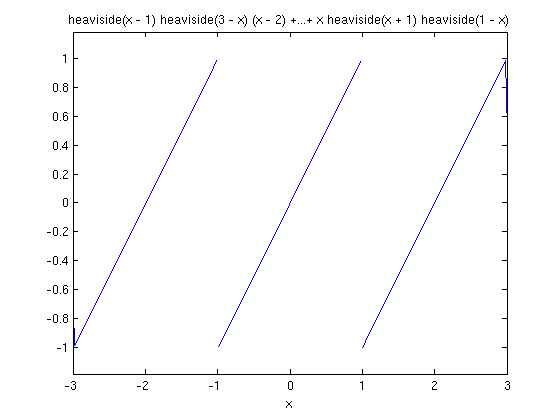
extends to be periodic on ![$[-3,3]$](fourier_series2_eq92526.png) , with period 2. To check that we've extended it correctly, we plot it.
, with period 2. To check that we've extended it correctly, we plot it.
ezplot(f,-3,3)
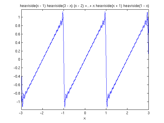
Here is a plot of the function and its Fourier series.
ezplot(fs(f,x,20,1),-3,3)
hold on
ezplot(f,-3,3)
hold off
It is somewhat clearer if the plots aren't the same color, so I'll use plot for the partial sum.
X = -3:0.001:3;
g = inline(vectorize(fs(f,x,20,1)));

ezplot(f,-3,3)
hold on
plot(X,g(X),'r')
hold off
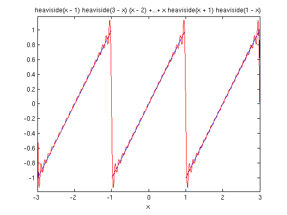
The overshoots are at the discontinuities of the 2 periodic extension of f. This is called the Gibbs Phenomenon.