As an example of using plyr for an analysis that requires a lot of data manipulation, we consider a problem in understanding career performance in baseball players. Trying to project future performance of players is relevant to many in the profession, specifically, a team manager negotiating a multi-year contract and a player's agent. If we consider a player requesting a long-term contract who is 8 years in the league and has been a top home run hitter for a couple of years. How do we project his performance 5-10 years hence?
Intialize the plyr package.
library(plyr)
The Lahman package provides datasets of baseball statistics.
library(Lahman)
str(Batting)
## 'data.frame':    93955 obs. of  24 variables:
##  $ playerID : chr  "aardsda01" "aardsda01" "aardsda01" "aardsda01" ...
##  $ yearID   : int  2004 2006 2007 2008 2009 2010 1954 1955 1956 1957 ...
##  $ stint    : int  1 1 1 1 1 1 1 1 1 1 ...
##  $ teamID   : Factor w/ 149 levels "ALT","ANA","ARI",..: 116 35 33 16 115 115 79 79 79 79 ...
##  $ lgID     : Factor w/ 7 levels "AA","AL","FL",..: 5 5 2 2 2 2 5 5 5 5 ...
##  $ G        : int  11 45 25 47 73 53 122 153 153 151 ...
##  $ G_batting: int  11 43 2 5 3 4 122 153 153 151 ...
##  $ AB       : int  0 2 0 1 0 0 468 602 609 615 ...
##  $ R        : int  0 0 0 0 0 0 58 105 106 118 ...
##  $ H        : int  0 0 0 0 0 0 131 189 200 198 ...
##  $ X2B      : int  0 0 0 0 0 0 27 37 34 27 ...
##  $ X3B      : int  0 0 0 0 0 0 6 9 14 6 ...
##  $ HR       : int  0 0 0 0 0 0 13 27 26 44 ...
##  $ RBI      : int  0 0 0 0 0 0 69 106 92 132 ...
##  $ SB       : int  0 0 0 0 0 0 2 3 2 1 ...
##  $ CS       : int  0 0 0 0 0 0 2 1 4 1 ...
##  $ BB       : int  0 0 0 0 0 0 28 49 37 57 ...
##  $ SO       : int  0 0 0 1 0 0 39 61 54 58 ...
##  $ IBB      : int  0 0 0 0 0 0 NA 5 6 15 ...
##  $ HBP      : int  0 0 0 0 0 0 3 3 2 0 ...
##  $ SH       : int  0 1 0 0 0 0 6 7 5 0 ...
##  $ SF       : int  0 0 0 0 0 0 4 4 7 3 ...
##  $ GIDP     : int  0 0 0 0 0 0 13 20 21 13 ...
##  $ G_old    : int  11 45 2 5 NA NA 122 153 153 151 ...
str(Master)
## 'data.frame':    17674 obs. of  35 variables:
##  $ lahmanID    : int  1 2 3 4 5 6 7 8 9 10 ...
##  $ playerID    : chr  "aaronha01" "aaronto01" "aasedo01" "abadan01" ...
##  $ managerID   : chr  NA NA NA NA ...
##  $ hofID       : chr  "aaronha01h" NA NA NA ...
##  $ birthYear   : int  1934 1939 1954 1972 1854 1877 1869 1866 1862 1874 ...
##  $ birthMonth  : int  2 8 9 8 11 4 11 10 3 10 ...
##  $ birthDay    : int  5 5 8 25 4 15 29 14 16 22 ...
##  $ birthCountry: chr  "USA" "USA" "USA" "USA" ...
##  $ birthState  : chr  "AL" "AL" "CA" "FL" ...
##  $ birthCity   : chr  "Mobile" "Mobile" "Orange" "West Palm Beach" ...
##  $ deathYear   : int  NA 1984 NA NA 1905 1957 1962 1926 1930 1935 ...
##  $ deathMonth  : int  NA 8 NA NA 5 1 6 4 2 6 ...
##  $ deathDay    : int  NA 16 NA NA 17 6 11 27 13 11 ...
##  $ deathCountry: chr  NA "USA" NA NA ...
##  $ deathState  : chr  NA "GA" NA NA ...
##  $ deathCity   : chr  NA "Atlanta" NA NA ...
##  $ nameFirst   : chr  "Hank" "Tommie" "Don" "Andy" ...
##  $ nameLast    : chr  "Aaron" "Aaron" "Aase" "Abad" ...
##  $ nameNote    : chr  NA NA NA NA ...
##  $ nameGiven   : chr  "Henry Louis" "Tommie Lee" "Donald William" NA ...
##  $ nameNick    : chr  "Hammer,Hammerin' Hank,Bad Henry" NA NA NA ...
##  $ weight      : int  180 190 190 184 192 170 175 169 190 180 ...
##  $ height      : num  72 75 75 73 72 71 71 68 71 70 ...
##  $ bats        : chr  "R" "R" "R" "L" ...
##  $ throws      : chr  "R" "R" "R" "L" ...
##  $ debut       : Date, format: "1954-04-13" "1962-04-10" ...
##  $ finalGame   : Date, format: "1976-10-03" "1971-09-26" ...
##  $ college     : chr  NA NA "Cal St. Fullerton" "Middle Georgia JC" ...
##  $ lahman40ID  : chr  "aaronha01" "aaronto01" "aasedo01" "abadan01" ...
##  $ lahman45ID  : chr  "aaronha01" "aaronto01" "aasedo01" "abadan01" ...
##  $ retroID     : chr  "aaroh101" "aarot101" "aased001" "abada001" ...
##  $ holtzID     : chr  "aaronha01" "aaronto01" "aasedo01" "abadan01" ...
##  $ bbrefID     : chr  "aaronha01" "aaronto01" "aasedo01" "abadan01" ...
##  $ deathDate   : Date, format: NA "1984-08-16" ...
##  $ birthDate   : Date, format: "1934-02-05" "1939-08-05" ...
These are yearly total stats for players spanning the years:
min(Batting$year)
## [1] 1871
max(Batting$year)
## [1] 2010
Being a Hall of Fame player is based on a whole career of performance. The data are given per year and per player. To get career-long home run statistics we need to group the data by player and analyze total statistics for each player's sub-data.frame.
hr_stats_df <- ddply(Batting, .(playerID), function(df) c(mean(df$HR, na.rm = T),
    max(df$HR, na.rm = T), sum(df$HR, na.rm = T), nrow(df)))
head(hr_stats_df)
##    playerID     V1 V2  V3 V4
## 1 aardsda01  0.000  0   0  6
## 2 aaronha01 32.826 47 755 23
## 3 aaronto01  1.857  8  13  7
## 4  aasedo01  0.000  0   0 13
## 5  abadan01  0.000  0   0  3
## 6  abadfe01  0.000  0   0  1
nrow(hr_stats_df)
## [1] 17453
names(hr_stats_df)[c(2, 3, 4, 5)] <- c("HR.mean", "HR.max", "HR.total", "career.length")
Our player of interest has been around for 8 years and is requesting a multi-year contract, so let's restrict our attention to players that were in the league for at least 10 years.
hr_stats_long_df <- subset(hr_stats_df, career.length >= 10)
Let's merge this data into the Batting data.frame so we have the other information to work with, too.
Batting_hr <- merge(Batting, hr_stats_long_df)
This both merged the data and restricted the players to the ones we identified with at least 10 years in the game.
In order to analyze how players perform over their careers using this yearly data we need to know which career-year a given year's record corresponds to. Let's look at one player and define a new variable that indicates this. Babe Ruth has playerID "ruthba01".
ruth_df <- subset(Batting_hr, playerID == "ruthba01")
min(ruth_df$yearID)
## [1] 1914
ruth_df2 <- transform(ruth_df, career.year = yearID - min(yearID) + 1)
head(ruth_df2)
##       playerID yearID stint teamID lgID   G G_batting  AB   R   H X2B X3B
## 38476 ruthba01   1931     1    NYA   AL 145       145 534 149 199  31   3
## 38477 ruthba01   1918     1    BOS   AL  95        95 317  50  95  26  11
## 38478 ruthba01   1932     1    NYA   AL 133       133 457 120 156  13   5
## 38479 ruthba01   1915     1    BOS   AL  42        42  92  16  29  10   1
## 38480 ruthba01   1934     1    NYA   AL 125       125 365  78 105  17   4
## 38481 ruthba01   1933     1    NYA   AL 137       137 459  97 138  21   3
##       HR RBI SB CS  BB SO IBB HBP SH SF GIDP G_old HR.mean HR.max HR.total
## 38476 46 163  5  4 128 51  NA   1  0 NA   NA   145   32.45     60      714
## 38477 11  66  6 NA  58 58  NA   2  3 NA   NA    95   32.45     60      714
## 38478 41 137  2  2 130 62  NA   2  0 NA   NA   133   32.45     60      714
## 38479  4  21  0 NA   9 23  NA   0  2 NA   NA    42   32.45     60      714
## 38480 22  84  1  3 104 63  NA   2  0 NA   NA   125   32.45     60      714
## 38481 34 103  4  5 114 90  NA   2  0 NA   NA   137   32.45     60      714
##       career.length career.year
## 38476            22          18
## 38477            22           5
## 38478            22          19
## 38479            22           2
## 38480            22          21
## 38481            22          20
To do this uniformly for all players we use ddply to group the data by player, we add the career.year variable calculated for this player, then join all the data.frames together into one.
Batting_hr_cy <- ddply(Batting_hr, .(playerID), function(df) transform(df, career.year = yearID -
    min(yearID) + 1))
head(Batting_hr_cy)
##    playerID yearID stint teamID lgID   G G_batting  AB   R   H X2B X3B HR
## 1 aaronha01   1967     1    ATL   NL 155       155 600 113 184  37   3 39
## 2 aaronha01   1971     1    ATL   NL 139       139 495  95 162  22   3 47
## 3 aaronha01   1954     1    ML1   NL 122       122 468  58 131  27   6 13
## 4 aaronha01   1965     1    ML1   NL 150       150 570 109 181  40   1 32
## 5 aaronha01   1960     1    ML1   NL 153       153 590 102 172  20  11 40
## 6 aaronha01   1955     1    ML1   NL 153       153 602 105 189  37   9 27
##   RBI SB CS BB SO IBB HBP SH SF GIDP G_old HR.mean HR.max HR.total
## 1 109 17  6 63 97  19   0  0  6   11   155   32.83     47      755
## 2 118  1  1 71 58  21   2  0  5    9   139   32.83     47      755
## 3  69  2  2 28 39  NA   3  6  4   13   122   32.83     47      755
## 4  89 24  4 60 81  10   1  0  8   15   150   32.83     47      755
## 5 126 16  7 60 63  13   2  0 12    8   153   32.83     47      755
## 6 106  3  1 49 61   5   3  7  4   20   153   32.83     47      755
##   career.length career.year
## 1            23          14
## 2            23          18
## 3            23           1
## 4            23          12
## 5            23           7
## 6            23           2
To get deeper information about top career players it'll be helpful to analyze the most recent players and Hall of Fame players from the past. To this end, we'll segregate players that started before 1940 from those that started after 1950. This requires tagging each player with the starting year. We'll add a column to the data.frame with this information as follows.
start_year_df <- ddply(Batting_hr_cy, .(playerID), function(df) min(df$yearID))
head(start_year_df)
##    playerID   V1
## 1 aaronha01 1954
## 2  aasedo01 1977
## 3 abbated01 1897
## 4 abbotgl01 1973
## 5 abbotji01 1989
## 6 abbotku01 1993
names(start_year_df)[2] <- "start.year"
# Merge this with other data.
Batting_hr_cy2 <- merge(Batting_hr_cy, start_year_df)
Now we select subframes of players with separate starting years.
Batting_early <- subset(Batting_hr_cy2, start.year < 1940)
Batting_late <- subset(Batting_hr_cy2, start.year > 1950)
Let's get the top 10 home run hitters in the early group and the late group. We could order our Batting data.frames by total home runs, but we'd have lots of rows for each player (one for each year played). It's simpler to form a new dataframe that just has the total home runs per player.
tot_HR_early <- subset(Batting_early, select = c(playerID, HR.total))
head(tot_HR_early, n = 3)
##     playerID HR.total
## 37 abbated01       11
## 38 abbated01       11
## 39 abbated01       11
# Remove the duplicate rows:
tot_HR_early <- unique(tot_HR_early)
head(tot_HR_early, n = 3)
##      playerID HR.total
## 37  abbated01       11
## 172 adamsba01        3
## 206 adamssp01        9
Now we want to sort this data.frame by total homeruns in descending order. The plyr package provides a nice function to do this, called arrange.
tot_HR_early_srt <- arrange(tot_HR_early, desc(HR.total))
head(tot_HR_early_srt, n = 3)
##    playerID HR.total
## 1  ruthba01      714
## 2  foxxji01      534
## 3 willite01      521
top10_HR_hitters_early <- tot_HR_early_srt[1:10, "playerID"]
Now repeat this for the later players.
tot_HR_late <- subset(Batting_late, select = c(playerID, HR.total))
# Remove the duplicate rows:
tot_HR_late <- unique(tot_HR_late)
tot_HR_late_srt <- arrange(tot_HR_late, desc(HR.total))
head(tot_HR_late_srt, n = 3)
##    playerID HR.total
## 1 bondsba01      762
## 2 aaronha01      755
## 3  mayswi01      660
top10_HR_hitters_late <- tot_HR_late_srt[1:10, "playerID"]
First restrict the Batting data to these players.
Batting_early_top10 <- subset(Batting_early, playerID %in% top10_HR_hitters_early)
To get a sense of how home run performance varies over the career, let's just plot that data. To exclude any anomalies due to time injured and not playing we'll plot the ratio of home runs over at bats per year instead of the raw home run numbers.
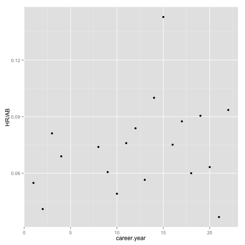
To begin, plot this for willite01.
library(ggplot2)
ggplot(data = subset(Batting_early_top10, playerID == "willite01"), aes(x = career.year,
    y = HR/AB)) + geom_point()
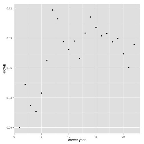
How does Babe Ruth look?
ggplot(data = subset(Batting_early_top10, playerID == "ruthba01"), aes(x = career.year,
    y = HR/AB)) + geom_point()
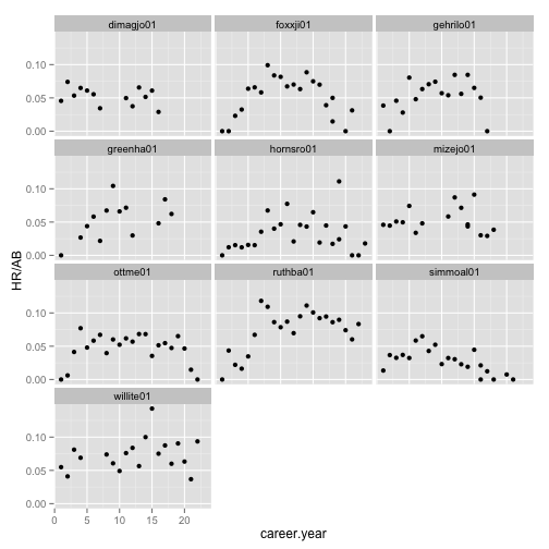
We can get a view of the performance of all ten players using a facet plot.
ggplot(data = Batting_early_top10, aes(x = career.year, y = HR/AB)) + geom_point() +
    facet_wrap(~playerID, ncol = 3)
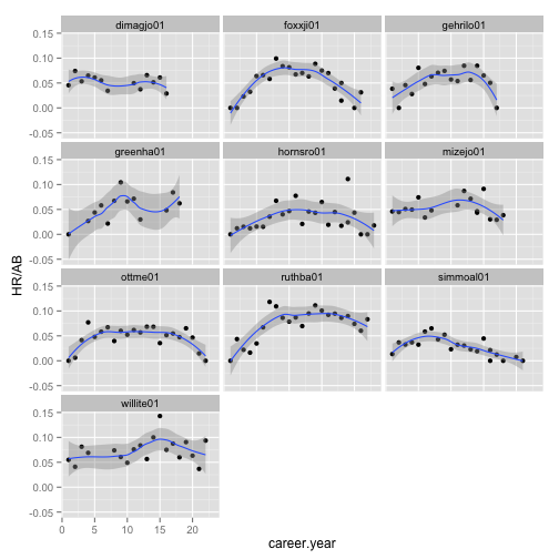
We can get a sense of the trends by adding a loess fit line to the panel.
ggplot(data = Batting_early_top10, aes(x = career.year, y = HR/AB)) + geom_point() +
    facet_wrap(~playerID, ncol = 3) + geom_smooth()
First restrict the Batting data to these players.
Batting_late_top10 <- subset(Batting_late, playerID %in% top10_HR_hitters_late)
Let's jump to the final facet plot.
ggplot(data = Batting_late_top10, aes(x = career.year, y = HR/AB)) + geom_point() +
    facet_wrap(~playerID, ncol = 3) + geom_smooth()
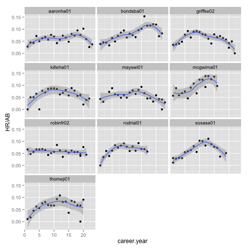
In most players their skills declined after about 10-12 years or stayed flat. Also, they tend to climb to a plateau early (7-8 years). Steep linear power growth for 10 years and late decline in skills is characteristic of players significantly associated with steroid use (Barry Bonds, Mark McGwyer, Sammy Sosa). We don't see the same picture in Alex Rodriguez, who did take steroids, so nothing is certain.