|
|
|
|
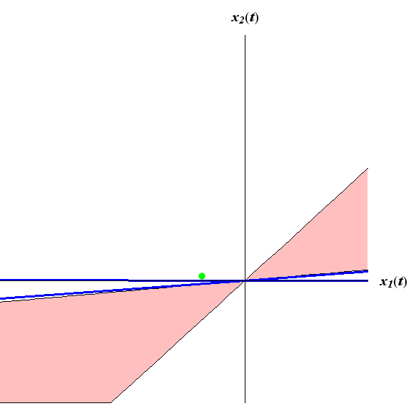
Animation 1: |
Animation 2: |
Animations for
"Non-autonomous linear differential equations"
Click on thumbnails to view animations or the .nb links for Mathematica code to produce the animations.
|
|
|
|
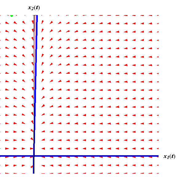
Animation 1: |
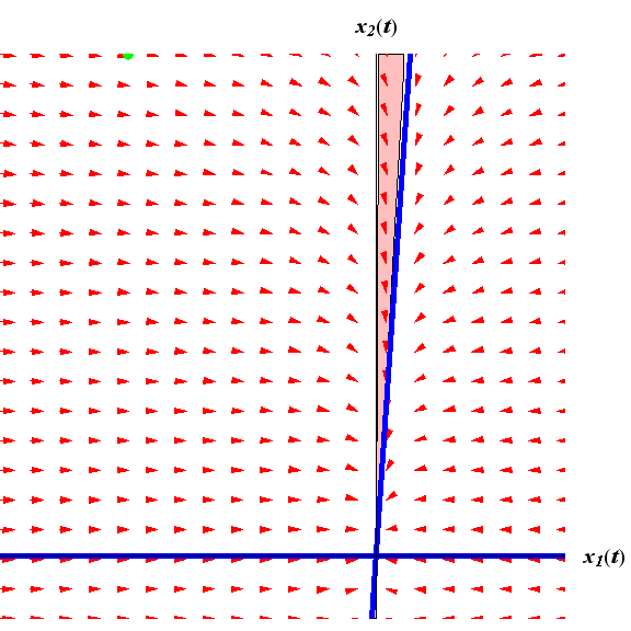
Animation 2: |
|
|
|
|
Animation 3: |
Animation 4: |
|
|
|
Animation 5: |
|
|
|
|
Animation 6: |
Animation 7: |