Goal: This case introduces the two "naive" forecasting models introduced in Chapter One applied to forecasting stock rates of return. Specifically, it introduces

• How to access data in FORECASTX^TM
• How to generate simple forecasts of stock returns using Excel
• How to judge the relative accuracy of forecasting models
• FORECASTX^TM basics such as Procast^TM
• The random walk hypothesis of the stock market.

The spreadsheet for this problem is CH1_Case1.xls. It contains the following data:

The series FSPCOM is the monthly S&P 500 Composite Stock Index.

The series %FSPCOM is the percentage change in the S&P 500 composite index over the period. This was computed using a spreadsheet as follows:

Here we have used a log transformation converting our stock index data into continuously compounded rates of return, i.e., interest is assumed to be paid continuously over any period. Continuously compounding is a common assumption in the finance literature as opposed to annual or discrete compounding.

The series FORECAST_ONE contains forecasts of %FSPCOM using the first-naïve forecasting model of Chapter One. The first naive or simplest forecasting model uses the previous actual value of a variable A_t-1 as a forecast for the next period F_t:

F_t = A_t-1

Here, our forecast for next period is what we observe today. While we call this model "naive," in fact it represents the correct model for forecasting a martingale process and the so-called "Law of Iterated Expectations," in which forecasts of martingales depend only on current information.

The series FORECAST_TWO contains forecasts of %FSPCOM using the second-naïve forecasting model of Chapter One. This second "naive" forecasting model adds an adaptive structure to the former model:

F_t = A_t-1 + P(A_t-1 - A_t-2)

where F_t is the forecast for period t, A_t-1 is the actual observation at period t-1, A_t-2 is the observed value at period t-2, and P is a parameter determining the proportion of the change between periods t-2 and t-1. Such a model is called autoregressive since forecasts depend on several lagged values of the variable in question. The values for FORECAST_TWO were generated with assuming P = .5.

To view a time-series plot of each series select the cells containing the series in Excel and then click on the FORECASTX^TM icon on the Excel toolbar. The "Data Capture" screen should now appear. Next select the Forecast Method menu and click on the Preview button to see a time-series plot of the selected series. You can then print the graph from this screen.

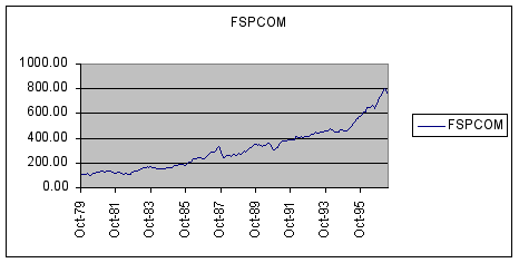
Using Excel’s Chart Wizard a plot of FSPCOM for our sample period is shown below. (Note the abrupt drop in October of 1987!)

Question #1: Based upon examination of the time-series plot of FSPCOM, do stock prices show an appreciable trend over time?

ANSWER:

Modern financial theory, however, focuses on rates-of-return rather than the stock price. Accordingly, the variable we wish to forecast is %FSPCOM.

Using Excel’s Chart Wizard a plot of %FSPCOM for our sample period is shown below. (Note again the sharp drop in October of 1987.)

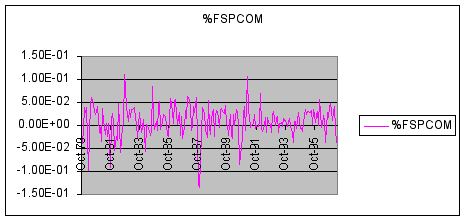
Question #2: Based upon examination of the time-series plot of %FSPCOM, do stock rates of return show an appreciable trend?

ANSWER:

The theory of efficient capital markets argues that stock prices incorporate all relevant information immediately and therefore there is no useful information in past patterns of stock prices. This implies a martingale property of stock returns, which asserts that the best forecast of today’s rate of return conditional on current information is yesterday’s actual return (the first-naïve forecasting model). This martingale property of stock returns underlies much of modern asset-pricing theory in finance.

Fortunately, the two "naive" forecasting models presented in Chapter One provide the basis for a simple test of the random walk hypothesis. Specifically, the first naive forecasting model implies that all adjustment in stock prices to new information occur immediately, consistent with the random walk model. If, however, stock prices take time to adjust to new information, then information beyond last period's return may be useful. We can examine this assertion by including an adaptive mechanism (to the first-naïve model above), which is the second naive forecasting model of Chapter One.

Using Excel, we calculated forecasts using the second naïve forecasting model (FORECAST_TWO) as follows:

This forecasting model adds an adaptive structure to the first naïve model. Note, we have set the value of the parameter P at .5 for this application, where 0 £ P £ 1.

If the random walk model is correct, the addition of information beyond last period's actual rate of return should be useless in forecasting a martingale process and they should result in enhanced forecasting error. Accordingly, we expect the root-mean-square-error (RMSE) for the first-naïve model to be less than that of the second when applied to stock rates of return since it ignores information beyond last period. Accordingly, we can test for a random walk in the context of the two naive forecasting models of Chapter One.

Note: Calculating naïve forecasts reduce the range of the forecast series relative to the original series. This is due to autoregressive forecasting algorithms being applied to a fixed sample. Accordingly, FORECAST_TWO requires more data since it postulates a longer autoregressive lag process in the data.

A plot of the two forecast series and actual returns for 1996 is shown below:

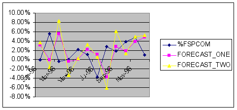
Note how the first naive model mirrors exactly the original series, with a one-period lag. The second-naive model behaves differently due to its adaptive structure. Note also the large errors in 1996M3 and 1996M8 in the second forecasting model, relative to the first model.

A similar plot for the entire sample is reported below.

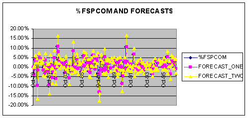
From the plot above it is clear that FORECAST_TWO is more variable than FORECAST_ONE is tracking %FSPCOM.

Finally, to examine statistically which forecasting model gives the better fit over the sample period, we compute goodness-of-fit statistics between the actual and forecasted series. Specifically, using Excel we calculated root-mean-squared error for each of the two forecasting models, which are reported in the Table below. (These are calculated in the spreadsheet to this case: CH1_Case1.xls)

Question #3: Based upon examination of RMSE, which forecasting method is more accurate over the period 1980M1-1997M4?

ANSWER:

Question #4: Is your answer to Question 3 consistent with stock returns following the random-walk hypothesis, i.e., that past patterns of stock rates of return are irrelevant in forecasting future returns?

ANSWER:

The Procast^TM application in FORECASTX^TM is an expert selection one-step forecasting tool that is designed to determine the best forecasting technique for a given data series. To see if Procast^TM can shed any light on the issue of this case we applied Procast^TM to the %FSPCOM series with the following forecast results for the single period of August of 1997:

Note that expert selection driver choose Holt-Winters smoothing as the optimal forecast method. This suggests that the %FSPCOM series is nonstationary contradicting our previous results. While this may be of some concern, it is quite common in forecasting applications. Accordingly, one may question blind use of expert selection software. For example, from the printed reports we see that the alpha parameter and the gamma parameter are both set equal to zero by the software in calculating forecasts using Holt-Winters smoothing. This suggests the model is being constrained by the range of the parameters. The point is simple: Be careful of blindly following the results of expert selection software without understanding the underlying statistics and model. Nevertheless, students should be impressed how well the first-naïve forecasting model does relative the more-sophisticated Holt-Winters model!

Question #1: This assignment concluded that, for %FSPCOM, the first-naive model outperformed the second-naive model. This however, assumed an adjustment parameter of P = 0.5, and a one-period ahead forecast horizon using data from the period 1979-1980. The important question is how robust are our findings given these assumptions? Specifically, try altering the parameter P, the forecast horizon, and the sample period to see if our results are sensitive to changes in these assumptions. For instance, are there some values of P in which the second-naive model outperforms the first? Discuss your findings!

Question #2: Try redoing this assignment with a different portfolio of stocks (AMEX, NASDAQ) or a single stock. Contrast and compare your results with those reported in the case.