Goal: This case employs data-smoothing techniques used to track and forecast the Standard and Poors 500 Stock Market Index emphasizing model selection procedures. Specifically, this case introduces:

• Model Selection regarding Data Trend and Stationarity
• Generating Forecasts using various Smoothing Techniques
• Procedures for Analyzing Out-of-Sample Forecast Accuracy

The spreadsheet for this problem is CH3_Case1.xls. It contains the following data:

The series FSPCOM is the monthly S&P 500 Composite Stock Index. Note the FSPCOM data are index numbers representing a value-weighted average of 500 stocks of major U.S. corporations.

The series %FSPCOM is the percentage change in the S&P 500 composite index over the period. This was computed using a spreadsheet as follows:

It is important to ascertain the time-series properties of our data, which will guide us in the model selection process. Specifically, preliminary data analysis for trend (stationarity), seasonality, and cyclical components should always be undertaken.

To visually view the data over the sample period we generated the following plot in Excel.

Question #1: Describe the time-series plot of FSPCOM, noting any significant trend or seasonality.

ANSWER:

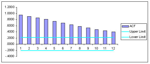
A formal way to test for data stationarity in FORECASTX^TM is to estimate the autocorrelation function and the related correlogram. To obtain ACF function estimates in FORECASTX^TM simply select the Analyze button in the Model Selection screen. This produces graphs of the ACF function, which you can save in an Excel spreadsheet.

Using FORECASTX^TM, we obtained the following autocorrelation estimates, followed by the correlogram for FSPCOM.

Question #2: Using the estimated ACF function, test whether the FSPCOM data are stationary.

ANSWER:

To complete this case we will want to examine forecast model accuracy out-of-sample, which is accomplished by use of a holdout period. Accordingly, we select our sample period to be from 1980M1-1985M12, whereas the holdout period will be from 1986M1-1986M12 for which we will generate forecasts based on the sample period to assess out-of-sample accuracy. Based upon this analysis we will select the optimal forecasting method.

Use of a holdout period is easily accomplished in FORECASTX^TM by using the Holdback Evaluation utility in FORECASTX^TM. Specifically, select columns labeled DATE and FSPCOM in CH3_Case1.xls and then enter FORECASTX^TM. In the Data Capture screen select yes on the Data Set Contains box. This tells FORECASTX^TM that dates are included in the data range. Next, on the Data Capture screen set the number of periods to forecast equal to zero (we will change this later in this case when we generate forecasts beyond 1986M12). We now select the Data Cleansing button, which takes you to the Advanced Options screen. There select the Use Holdback button in the Holdback Evaluation box. This tells FORECASTX^TM to treat a portion of the sample as a holdout period in which we can compare forecasts with actual values to assess model accuracy. For this case we select a holdback period of 12, which implies 1986M1-1986M12 is our holdback period.

Using the holdback procedure we compared three candidate models to forecast the S&P 500: Simple Exponential Smoothing, Adaptive Exponential Smoothing, and Holt-Winters Smoothing. As our S&P 500 data are nonstationary, we expect Holt-Winters to perform the best in the holdback period. Using FORECASTX^TM the following accuracy statistics were generated for the three models.

Here MAPE is mean absolute percentage forecast error, which measures the average absolute forecast error. SSE is the sum of squared errors used to calculate root-mean-squared-error (RMSE). These are accuracy statistics over the holdback period 1986M1-1986M12 and they show that Holt-Winters Smoothing has superior accuracy followed by Simple Exponential Smoothing and Adaptive Exponential Smoothing.

This result confirms our expectation that Holt-Winters Smoothing is the more appropriate model when dealing with nonstationary data as shown by RMSE. This can also be seen by the reports, which show that FORECASTX^TM attempts to set the optimal smoothing parameter equal to one in both cases, suggesting the models are trying to deal with a significant trend, which these models are not designed to deal with!

Technical analysts on Wall Street attempt to forecast the S&P 500 Index using various time-series methods. Here we will generate forecasts into 1997 using the three smoothing models: Simple Exponential Smoothing, Adaptive Exponential Smoothing, and Holt-Winters Smoothing.

One can easily generate forecasts for 1987M1-1987M12 using FORECASTX^TM. Specifically, select columns labeled DATE and FSPCOM in CH3_Case1.xls and then enter FORECASTX^TM. In the Data Capture screen select yes on the Data Set Contains box. This tells FORECASTX^TM that dates are included in the data range. Next, on the Data Capture screen set the number of periods to forecast equal to 12 (we are generating forecasts for 1987M1-1987M12). We now select the Data Cleansing button, which takes you to the Advanced Options screen. There de-select the Use Holdback button if it is on in the Holdback Evaluation box. This tells FORECASTX^TM to generate forecasts beyond the sample period 1980M1-1986M12. Proceed to the Forecast Selection screen and choose the appropriate model and gather the printed reports.

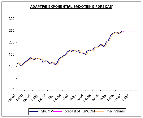
Plots of the three methods and their respective forecasts are shown below.

Question #3: Viewing the forecasts displayed above over 1987M1-1987M12, contrast and compare how each model generates forecasts. Why does Holt-Winters produce better forecasts?

ANSWER:

Question #1: Redo the assignment for the rate-of-returns data on the S&P 500. (This series is labeled %FSPCOM in the spreadsheet to this case.) Contrast and compare your results with those for FSPCOM.

Question #2: This case examined the sample period 1980M1-1986M12, where 1986 served as the holdout period. Redo the assignment for more recent data. How robust are the results of this case? Explain!