Goal: This case utilizes various smoothing techniques to forecast the civilian unemployment rate in the United States during the period 1975-1983, which includes the 1982 recession. Specifically, this case introduces

• Model Selection Procedures
• Generating Forecasts using Data Smoothing techniques
• Dealing with Cycles as a Cause of Nonstationarity
• Forecasting the Unemployment Rate.

The spreadsheet for this problem is CH3_Case2.xls. It contains the following data:

The series U_RATE is the seasonally adjusted monthly rate of unemployment.

Note that our data are seasonally adjusted, meaning that seasonal effects have been removed from the data. It is quite common to use seasonally adjusted data in empirical economics in that many models require non-seasonal data. On the other hand, we will later utilize forecasting models that explicitly account for data seasonality.

It is important to ascertain the time-series properties of our data, which will guide us in the model selection process. Since we are dealing with time series data, which are seasonally adjusted, i.e., seasonal effects have been removed, it is advised that we examine the data for trend and cycle components. In other words, are the data stationary? We can do this informally by viewing a time-series plot of the data, or we can test this assertion by estimating the sample autocorrelation function (ACF) and the associated correlogram.

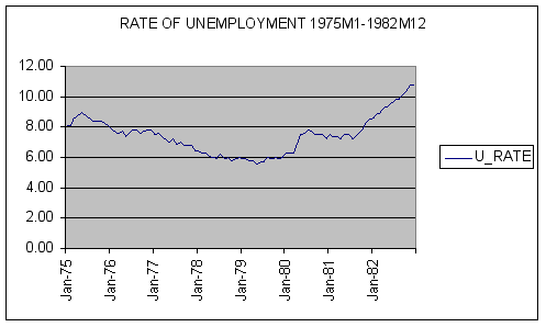
A plot the unemployment rate (U_RATE) over the sample period 1975M1-1982M12 is shown below.

Question #1: Based upon examination of the time-series plot of U_RATE, does the monthly unemployment data exhibit significant trend or pronounced cyclical variability?

ANSWER:

To formally test for data stationarity, we estimate the autocorrelation structure and associated correlogram using FORECASTX^TM. The estimation results and correlogram are reported below.

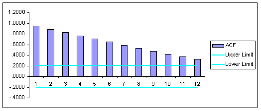
Question #2: Based upon the estimated autocorrelation structure, are the data stationary?

ANSWER:

To complete this case we will want to examine forecast model accuracy out-of-sample, which is accomplished by use of a holdout period. Accordingly, we select our sample period to be from 1975M1-1981M12, whereas the holdout period is 1982M1-1982M12 for which we will assess out-of-sample accuracy. Based upon this analysis we will select the optimal forecasting method.

A holdout period is easily accomplished in FORECASTX^TM by using the Holdback Evaluation utility. Specifically, select columns labeled DATE and U_RATE in CH3_Case2.xls and then enter FORECASTX^TM. In the Data Capture screen select yes on the Data Set Contains box. This tells FORECASTX^TM that dates are included in the data range. Next, on the Data Capture screen set the number of periods to forecast equal to zero (we will change this later in this case when we generate forecasts beyond 1982M12). We now select the Data Cleansing button, which takes you to the Advanced Options screen. There select the Use Holdback button in the Holdback Evaluation box. This tells FORECASTX^TM to treat a portion of the sample as a holdout period in which we can compare forecasts with actual values to assess model accuracy. For this case we select a holdback period of 12, which implies 1982M1-1982M12 is our holdback period.

Using the holdback procedure we compared three candidate models to forecast U_RATE: Moving Averages, Adaptive Exponential Smoothing, and Holt-Winters Smoothing. As our unemployment data are nonstationary, we expect adaptive or Holt-Winters smoothing to perform the best in the holdback period. Using FORECASTX^TM the following accuracy statistics were generated for the three models over the holdout period.

Here MAPE is mean absolute percentage forecast error, which measures the average absolute forecast error. SSE is the sum of squared errors used to calculate root-mean-squared-error (RMSE).

Question #3: Using RMSE, which forecasting method provides the best out-of-sample fit? Explain.

Answer:

To generate forecasts into 1983 using the three smoothing models: Moving Averages, Adaptive Exponential Smoothing, and Holt-Winters Smoothing.

One can easily generate forecasts for 1983M1-1983M12; select columns labeled DATE and U_RATE in CH3_Case2.xls and then enter FORECASTX^TM. In the Data Capture screen select yes on the Data Set Contains box. This tells FORECASTX^TM that dates are included in the data range. Next, on the Data Capture screen set the number of periods to forecast equal to 12 (we are generating forecasts for 1983M1-1983M12). We now select the Data Cleansing button, which takes you to the Advanced Options screen. There de-select the Use Holdback button if it is on in the Holdback Evaluation box. This tells FORECASTX^TM to generate forecasts beyond the sample period 1975M1-1982M12. Proceed to the Forecast Selection screen and choose the appropriate model and gather the printed reports.

Plots of the in-sample fit of the three methods and their respective forecasts are shown below.

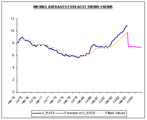
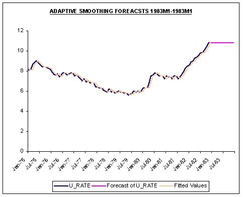
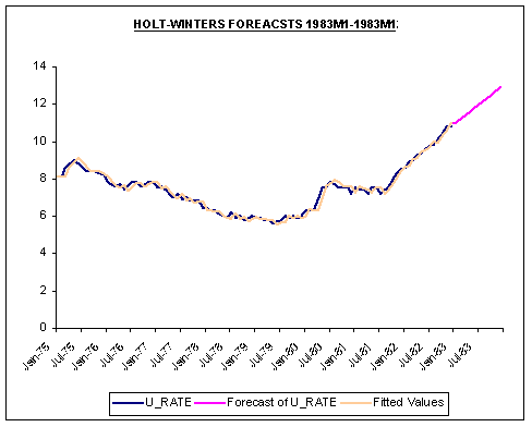
Question #4: Contrast and compare how each method generates forecasts for 1983. Which method do you have the most confidence?

Answer:

Question #1: How sensitive are the results of this case to the choice of the sample period? Explain!

Question #2: Redo this case using exchange rate data, e.g., the euro against the dollar. (Exchange rate data is easily obtainable on the WWW!) Contrast and compare your results.