Goal: This case examines the consequences of the common time-series problem of serial correlation (autocorrelation). Specifically, it introduces:

• Basic Keynesian Consumption Theory
• Testing for the presence of Autocorrelation
• Estimation of Autocorrelated Data using Data First-Differencing
• Implications of Spurious Regression.

The spreadsheet for this problem is CH4_Case2.xls. It contains the following data:

The series CON is quarterly data on Personal Consumption Expenditure (seasonally adjusted in current dollars). This variable measures aggregate consumption expenditure.

The series GNP is quarterly data on Gross National Product (seasonally adjusted in current dollars). This variable measures the total value of goods produced in the national economy.

The series DIFF_CON is the first difference of CON calculated as.

The series DIFF_GNP is the first difference of GNP calculated as above.

John Maynard Keynes, the father of modern macroeconomics, made two important theoretical observations about aggregate consumption behavior: (1) What was not consumed out of current income is saved; and (2) Current consumption depends on current income in a less than proportionate manner.

Keynes’ theories placed emphasis on a parameter called the marginal propensity to consume (MPC) which is the slope of the aggregate consumption function and a key factor in determining the "multiplier effect" of tax and spending policies.

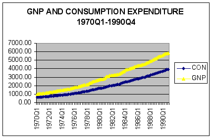
To examine behavior of personal consumption expenditure (CON) and gross national product (GNP) we generated a time-series plot in Excel.

Question #1: Based on examination of the time-series plot of CON and GNP, are these series stationary?

ANSWER:

To formally test whether both series are nonstationary, we estimated the autocorrelation function using the Analyze button in FORECASTX^TM.

Correlograms for CON and GNP are reported below.

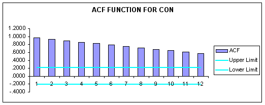
Question #2: Based on examination of the correlogram for each series, are the data stationary, i.e., can we reject all nulls of zero autocorrelation for a twelve-quarter lag structure at the 5-percent level of significance?

ANSWER:

Next, to examine the relationship between consumption and income, we estimated the correlation matrix for the two series using FORECASTX^TM.

Using Excel, a scatterplot of the data in levels is shown below.

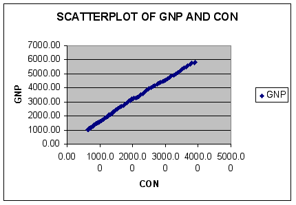
Question #3: Given the scatterplot and the estimated correlation between CON and GNP, do the two series appear to be related?

ANSWER:

Keynes’ analysis of the economy placed great emphasis on the size of the marginal propensity to consume (MPC), which determined the "multiplier effect" associated with fiscal and monetary policy. Keynes argued that the MPC was less than, but close to one.

We can obtain an estimate of the MPC by applying Ordinary Least Squares to the following aggregate consumption function:

GC = a + bGNP + e

where the slope parameter (b) is the marginal propensity to consume.

Estimation results of the Keynesian consumption function using FORECASTX^TM are reported below.

Question #4: How well does this model fit the data? Explain!

ANSWER:

The forecaster should be suspicious however that these results may be overly optimistic. The reason is that both series are nonstationary and therefore may have a common trend. In other words, the regression may be plagued by serial correlation.

Using FORECASTX^TM, we obtained the following estimate of the Durbin-Watson statistic.

Question #5: Does the data exhibit autocorrelation? Specifically, test the null hypothesis of no autocorrelation using the Durbin-Watson test.

ANSWER:

When significant autocorrelation is present, spurious regression may arise in that our results appear to be highly accurate when in fact they are not, since the OLS estimator of the regression error variance is biased downward. To investigate this possibility, we will re-estimate our consumption function using first differences of the original data. This transformation is designed to eliminate any common linear trend in the data.

A scatterplot of the transformed series DIFF_CON and DIFF_GNP is shown below.

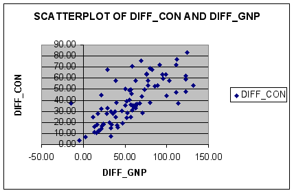
Note how the relationship between DIFF_CON and DIFF_GNP is still positive it is much more random than CON and GNP.

To test for stationarity in the first-differences of the data we produced the following correlograms using FORECASTX^TM.

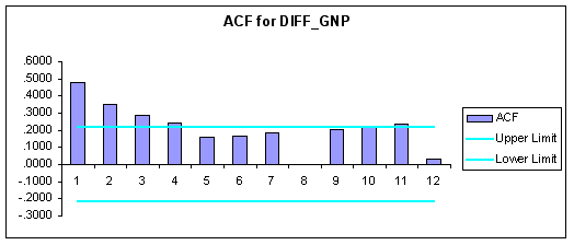
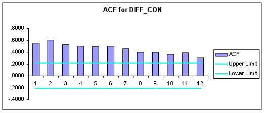
Question #6: Based upon the correlograms above are the first-differenced series stationary?

ANSWER:

Using FORECASTX^TM, the following results were obtained from estimating the consumption function using DIFF_CON and DIFF_GNP.

Question #7: How well does the revised model fit the data? Explain!

ANSWER:

To examine whether serial correlation is still a problem we estimated the Durbin-Watson statistic for the revised model.

Question #8: By reference to the Durbin-Watson statistic, does the revised model exhibit autocorrelation? Specifically, test the null hypothesis of no autocorrelation using the Durbin-Watson test.

ANSWER: Given K = 1 and N = 84, Table 4-7 gives us:

dL = 1.62 and dU = 1.67.

Given d = 1.76, by application of Figure 4-12 leads us to conclude that we no longer have autocorrelation, i.e., we cannot reject the null in favor of positive autocorrelation.

Question #9: Compare the estimated coefficient of determination (R2), the estimated coefficient on the independent variable, the standard error of the estimated coefficient on the independent variable, and t-values for both versions of the model.

Does the original model in levels (CON and GNP) show signs of spurious regression? Explain.

ANSWER: Comparisons of the two models are summarized below:

As we expect to find under autocorrelation, the two coefficient estimates are rather close, reflecting the fact that OLS slope estimator is still unbiased under autocorrelation, i.e., the slope estimates should converge for vary large samples.

On the other hand, the estimated standard error of the coefficient is much greater in the latter model than the former, consistent with OLS underestimating the regression variance in the first model. This is especially true for the t-statistics of the estimated slope coefficients, which differ by a factor of 200! Both of these results lead us to conclude that "Spurious Regression" plagues the first version of the model. In other words, the reported quality of our initial results is overstated.

Question #1: Explain why researchers should always check their regression models for the presence of serial correlation. What is "spurious" about this problem?

Question #2: Repeat the analysis of this case using second differences of CON and GNP. Contrast and compare your results to those of this case.