Goal: This assignment deals with the common problem of seasonality in time series data.

Specifically, it introduces:

• How to examine Data for Seasonality
• How to model Seasonality using Dummy Variables
• Analysis of an important Leading Economic Indicator, New Home Sales.

The spreadsheet for this problem is CH5_Case2.xls. It contains the following data:

The series N_HOME_SALES is monthly data on new homes sales in the United States.

The series TIME is an index taking the value of 1 in 1980M1 and increasing every year by a unit. This variable will proxy any linear growth over time in new homes sold.

The series M2-M12 are monthly seasonal dummy variables taking the value of one in their respective month. For example, the variable M5 takes the value of 1 in month five, and zero values elsewhere. The set of 11 dummies will allow us to quantify seasonal behavior in the context of multiple regression.

Seasonality is defined as variations in the level of data that occur with regularity at the same time each year. Accordingly, when the data are seasonal, we can use this information to improve our forecasts since, to a large extent, seasonal effects are predictable. For example, we can safely predict that ski lodges will have reduced business during the summer months.

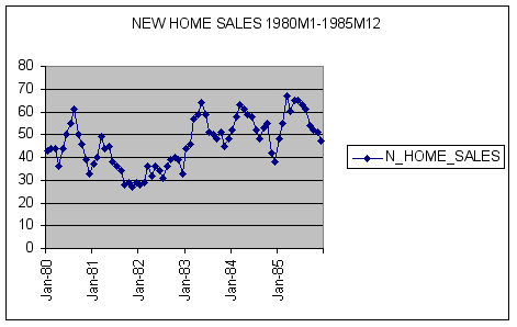
To visually inspect for seasonality, we plotted new homes sales data using Excel.

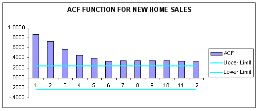
To formally test for data stationarity, we estimated a correlogram for N_HOME_SALES using FORECASTX^TM.

Question #1: Based upon examination of the time-series plot and correlogram of N_HOME_SALES, are the data seasonal? Explain.

ANSWER:

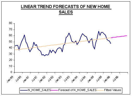
First, let’s estimate a linear trend model using 1985 as our holdout period to assess out-of-sample forecast accuracy as well as generate forecasts into 1986. This is easily done in FORECASTX^TM by using the holdback period button. The results are reported below in a series of tables.

The following accuracy statistics refer to the holdout period of 1985.

Question #2: How well does the linear trend model fit the data?

ANSWER:

Next we generated new home sales forecasts for the holdout period 1985M1-1985M12 as well as forecasts into 1986 based upon a linear trend model with seasonal dummies. Specifically, our forecasts will be based upon a model with two features:

1) Trend, accomplished by adding a time index to the model as an explanatory variable.

2) Season, accomplished by adding a series of seasonal dummies as explanatory variables. Here the dummy variables act as on-off switches for a certain time of the year for every year, allowing us to track seasonal variation in the regression model constant term. Accordingly, this approach handles seasonality in an additive manner.

Note: In creating our seasonal dummy variables, we have followed our "N-1" rule, as a set of 12 monthly seasonal dummy variables would be perfectly collinear.

The following multiple regression model designed to account for trend and data seasonality was estimated using FORECASTX^TM:

yt = a + bTIME + d2M2 + d3M3 + d4M4 + d5M5 + d6M6

+ d7M7 + d8M8 + d9M9 + d10M10 + d11M11 + d12M12 + e_t

Here the M2 through M12 are dummy variables with associated parameters d2, ...d12.

Accordingly, each dummy variable coefficient shows the level of housing sales in a given month relative to January, the base period.

The following accuracy statistics refer to the holdout period of 1985.

Question #3: Based upon the regression results above, do the pattern of estimated coefficients of the eleven dummy variables make sense? Which month has the highest new houses sold and which month the lowest? Explain noting the interpretation of the estimated parameters of the dummy variables.

ANSWER:

Question #4: Comment on how each model generates forecasts for 1996. Which method shows seasonality in forecasts for 1996?

ANSWER:

Question #1: Examine the seasonal linear time trend model (See Question #2) for the presence of serial correlation. Re-estimate the data using first differences of the data. Contrast and compare your results with those in this case.

Question #2: Try forecasting N_HOME_SALES using Winter's Exponential Smoothing. Contrast and compare your results with those of this case. Explain.