Goal: This case introduces time series decomposition in the context of forecasting the federal budget deficit for 1997, a time of transition from deficit to surplus in the United States. Specifically, this case introduces

• Deseasonalizing Data using Centered Moving Averages
• Estimating the Centered Moving Average Trend
• Generating Time Series Decomposition Forecasts using FORECASTX^TM
• Analysis and Forecasting the Federal Budget Surplus (Deficit)
• Expert Selection Forecasts using Procast^TM.

The spreadsheet for this problem is CH6_Case1.xls. It contains the following data:

The series BUDGET is the non-seasonally adjusted monthly federal budget surplus (deficit). The series is the "official" federal budget numbers from the Congressional Budget Office defined on a current account basis.

(The federal government does not officially maintain a capital account!)

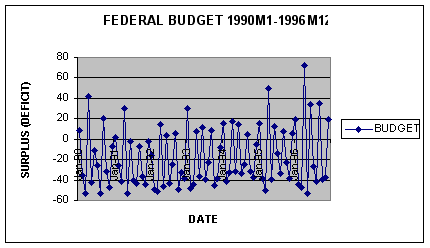
To get an idea of the behavior of the monthly deficit data over the historical period (1990M1-1996M12) we generated a time-series plot of the data using Excel. In addition, we generated autocorrelation statistics on BUDGET for a 12-month lag structure using the Analyze button in FORECASTX^TM.

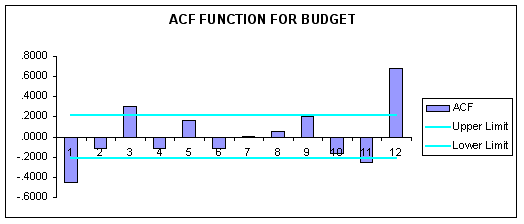
Question #1: Viewing the time-series plot and correlogram of the data, what behavior characterizes the data? Test for seasonality at various lags.

ANSWER:

Using FORECASTX^TM, one can easily obtain estimates of the time-series components of BUDGET by selecting Decomposition in the Forecasting Technique box. Click Multiplicative and select Linear Regression as the forecast method for decomposed data. From the reports we are able to extract the following components: centered moving average, centered moving average trend, seasonal factors, seasonal indices, and cycle factors, as well as forecasts of BUDGET.

Time series decomposition requires that we must first smooth away any seasonal and irregular variation, which is accomplished by calculating a centered moving average (CMA) of the BUDGET series. This smoothed (deseasonalized) series is then used to generate linear trend forecasts called the centered-moving-average trend (CMAT).

Using Excel we plotted the original, centered moving-average, and centered-moving-average trend series as shown below. In addition, we generated a correlogram for the CMA series.

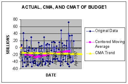
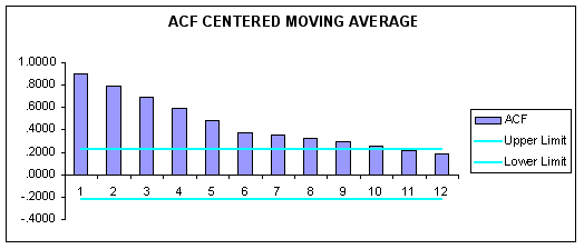
Question #2: Based upon examination of the time-series plot of BUDGET, CMA, and CMAT, contrast and compare the three series. Test for statistically significant seasonality in the CMA series using the estimated correlogram.

ANSWER:

The next step in the decomposition model is to extract the seasonal component from the data with the result being the creation of 12 seasonal index numbers to track seasonal effects into the forecast horizon. A plot of seasonal factors (calculated as the ratio of BUDGET to CMA for that period) generated by FORECASTX^TM is shown below.

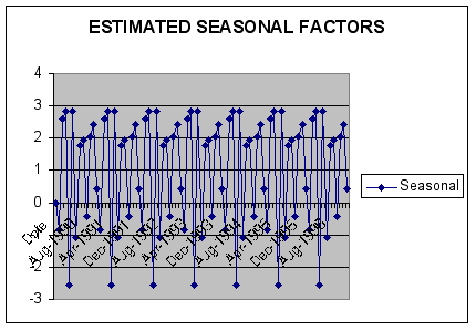
Based upon these estimated factors, FORECASTX^TM generated the following seasonal indices:

Note: What is the sum of the seasonal indices?

The seasonal indices used to forecast BUDGET into 1997 are plotted below.

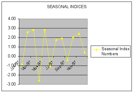
Question #3: Based upon examination of the 12 seasonal index numbers, are deficits seasonal? Explain.

ANSWER:

A major benefit of time-series decomposition is the ability to analyze and forecast data with a cyclical component. Since both government revenues and spending depend on the state of the economy we expect deficits to be cyclical -- deepening in recession relative to trend.

Using the Decomposition forecasting model, FORECASTX^TM calculates a series of cycle factors plotted in the following graph.

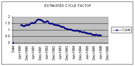
Question #4: How are cycle factors calculated? Describe the behavior of these factors over the sample period.

ANSWER:

Finally, to create the forecast numbers for the forecast period, we simply recombine the forecasted time-series components. Forecasts for 1997 using FORECASTX^TM are reported below.

The following graph plots forecasts for 1997 using time-series decomposition.

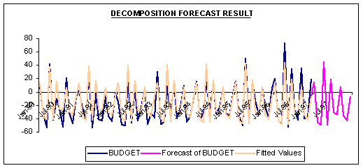
Question #5: What is your forecast for the federal budget deficit for 1997? Assess the accuracy of your forecast given the following actual budget values for the first four months of 1997: 13.36, -44.01, -21.32, 93.9, all in billions of dollars. Over the first four months of 1997, how accurate is our forecasting model?

ANSWER:

The following Table summarizes calculation of RMSE for the first-four months of 1997.

From the Table above we calculate RMSE to be 28.48, i.e., the average error expected each month is approximately 28 billion dollars. Accordingly, in any month this error can easily change a surplus to a deficit and vice-versa, showing how inaccurate our forecasts really are!

The following out-of-sample accuracy statistics were estimated for the holdout period 1986M1-1986M12 for the time series decomposition method.

We can use these holdback accuracy statistics to contrast and compare other potential forecasting models.

Let’s see how the Expert Selection feature of FORECASTX^TM handles the problem of forecasting the federal budget using the Procast^TM option. Simply select Procast in the Forecast Method menu and proceed to generate forecasts using 1986 as a holdback period and 1997 as the forecast horizon.

The method selected by Procast^TM is Holt-Winters Smoothing. Forecasts for 1997 and out-of-sample accuracy statistics are reported in the tables below.

Note the Holt-Winters forecast of the deficit for 1997 is -107 billion, about half of that of time series decomposition.

The following out-of-sample accuracy statistics were estimated for the holdout period 1986M1-1986M12 for the Holt-Winters Smoothing method.

Question #6: Comment on the method selected by FORECASTX^TM. What does this suggest about the time-series decomposition method applied to forecasting the federal budget surplus/deficit?

ANSWER:

Student Practice Question

Question #1: Redo the case using more recent data of the federal budget surplus (deficit), including the recent surpluses in 2001-2002. Contrast and compare your results with those of this case. Explain!