Goal: To examine complications when using time-series decomposition to generate forecasts of foreign car sales over a 20-year period. Specifically, we

• Critique the Time Series Decomposition Model
• Analyze Trend behavior in Foreign Car Sales
• Test differing versions of Time Series Decomposition using FORECASTX^TM.

The spreadsheet for this problem is C6_Case2.xls. It contains the following data:

The series FCS is quarterly foreign car sales (in 1000’s) in the United States.

You are a new hire at Ford Motor Company and you are assigned to the Business Forecasting unit. Your team is in charge of forecasting foreign car sales on a quarterly basis.

As part of your training, your boss asks you to forecast foreign car sales for 1996Q1-1996Q4, based upon historical data on foreign car sales (FCS) over the period 1975Q1-1995Q4. (Yes, this is historical data, but that’s the point! How well can you do using historical data)? She also requests that you employ time-series decomposition, since the model "mirrors the way upper management likes to think, and therefore generates credibility."

Question #1: Discuss why your boss may prefer time-series decomposition when presenting forecasts to upper-level management.

ANSWER: Your boss is probably concerned that forecasts appear to upper-level management as reasonable and useful rather than something generated by a "black box." Time-series decomposition, in the way it pieces apart sales data, is especially useful for many of the financial aspects of the firm. For example, firms use seasonality estimates to plan their working capital budgets and temporary hiring needs; the cyclical component relates firm sales to the health of the overall economy and macroeconomic factors such as gross domestic product, interest rates, and exchange rates. Finally, trend estimates are crucial for strategic long-term planning and capital budgeting. It is because of this intuitive application to sales forecasting that many financial analysts favor this model.

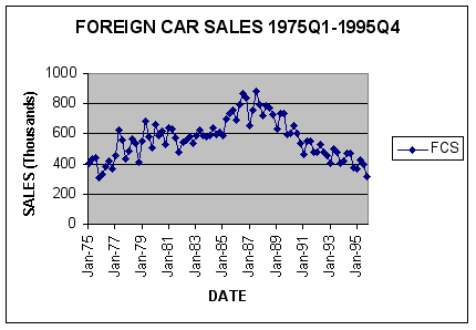
To get an idea of the behavior of the quarterly FCS data over the historical period (1975Q1-1995Q4) we generated a time-series plot of the data using Excel. In addition, we generated autocorrelation statistics on FCS for a 12-quarter lag structure using the Analyze button in FORECASTX^TM.

Question #2: Viewing the time-series plot and ACF correlogram of the data, what behavior characterizes the data? Are the data stationary?

ANSWER:

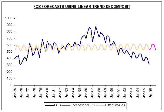
Using FORECASTX^TM, one can easily obtain estimates of the components of FCS and forecasts by selecting Decomposition in the Forecasting Technique box. Click Multiplicative and select Linear Regression as the forecast method for decomposed data. The following reports for FCS were obtained from FORECASTX^TM using 1995 as a holdout period and generating forecasts for 1996.

The following accuracy measures are for the holdout period 1995:

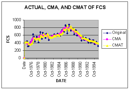
The following graph plots the actual data (FCS) along with the centered moving average (CMA) and the centered moving average trend (CMAT).

Question #3: Based upon the results above, how do you feel about your boss’s insistence on using time-series decomposition to forecast foreign car sales?

ANSWER:

Since the linear trend option of decomposition may not be appropriate for FCS we re-estimated the model using Exponential Smoothing to estimate the trend component.

Using FORECASTX^TM, select Decomposition in the Forecasting Technique box. Click Multiplicative and select Exponential Smoothing as the forecast method for decomposed data. The following reports for FCS were obtained from FORECASTX^TM for the smoothed trend decomposition model. Once again we used 1996 as the holdout period and 1997 as the forecast horizon.

The following accuracy measures are for the holdout period 1995:

Question #4: Contrast and compare the exponential trend version of the decomposition model with the linear trend version. Which model has the better out-of-sample accuracy over the holdout period?

ANSWER:

The following table summarized various accuracy statistics for the holdout period of 1995 for each respective model.

Clearly the exponential smoothing trend model has the ability to adapt to the trend reversal in the FCS data.

To investigate further you plot the estimated cycle factors for each approach as shown below:

Question #5: Based upon a plot of the historical cycle factors, do you see anything unusual?

ANSWER:

After some thinking you realize that foreign car sales may have been driven by two opposing forces: 1) an expanding U.S. economy, and 2) stiff quality and price competition from U.S. auto manufacturers. So you think to yourself, what is the plot telling you? There is a trend reversal in FCS around 1987.

Looking at this graph, the trend line is flat because we are combining periods of different consumer tastes and product quality. In other words, the actual trend is unstable over the entire sample period and is being forced into the cycle factors in the linear model.

Question #6: How’s your frustration level? What do you tell your boss?

ANSWER:

Question #1: Redo this assignment using domestic car sales as the dependent variable. Specifically, compare and contrast Winter's and Time Series Decomposition forecasts of domestic car sales data (See C6_Case2.xls). Compare and contrast your results with those of this case.