CHAPTER SEVEN
Case #14: TREND REVERSAL AND FOREIGN CAR SALES ONCE AGAIN
Goal: To examine the Box-Jenkins approach to forecasting foreign car sales. Specifically, we extend our analysis of foreign car sales found in Chapter Six, Case #2. In addition, this case introduces
Problem Spreadsheet
The spreadsheet for this problem is C7_Case2.xls. It contains the following data:
|
Variable |
Data Range |
|
FCS |
1975Q1-1995Q4 |
The series FCS is quarterly foreign car sales (in 1000’s) in the United States.
The Task Ahead
Once again, you are a new hire at Ford Motor Company and your boss asks you to forecast foreign car sales for 1996Q1-1996Q4 based upon historical data on foreign car sales (FCS) over the period 1975Q1-1995Q4. Given your experience with forecasting FCS using time series decomposition, you now seek to impress your new boss by investigating how ARIMA models perform over the holdout period 1995Q1-1995Q4. Your goal: Beat your boss’s time-series decomposition forecasts.
Examining the Data
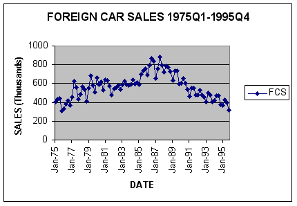
To examine the data for trend and seasonality, we generated a plot of foreign car sales over the sample period.

Question #1: Does the data exhibit significant trend and seasonality? What problems might the forecaster encounter using the linear version of the time series decomposition model?
ANSWER:
Examining the Data for Stationarity
The estimated ACF and PACF and associated correlograms for FCS are reported below.
|
Obs |
ACF |
PACF |
|
1 |
.8112 |
.8112 |
|
2 |
.6848 |
.0783 |
|
3 |
.7362 |
.4725 |
|
4 |
.7564 |
.1447 |
|
5 |
.5755 |
-.4171 |
|
6 |
.4629 |
-.1140 |
|
7 |
.5077 |
.1019 |
|
8 |
.5203 |
.1730 |
|
9 |
.3449 |
-.2249 |
|
10 |
.2662 |
-.0069 |
|
11 |
.2978 |
-.1168 |
|
12 |
.2539 |
-.1010 |
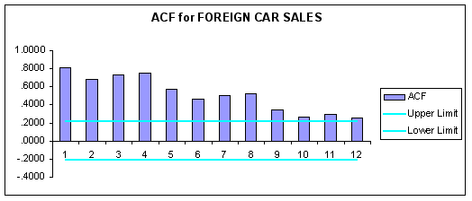
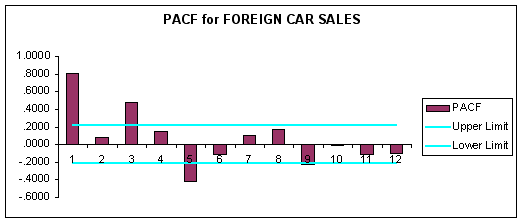
Question #2: Viewing the ACF and PACF, evaluate trend and seasonality in the data. Are the data stationary?
ANSWER:
Accordingly, some form of data transformation will be required to induce stationarity.
ARIMA Model Identification
Examining the ACF and PACF reported above, we see that the data will require some transformation before we can apply the Box-Jenkins methodology. Accordingly, we employed a first differencing transformation of the data in levels to remove any linear trend. The ACF and PACF of the first-differenced data are reported below.
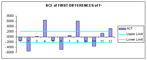
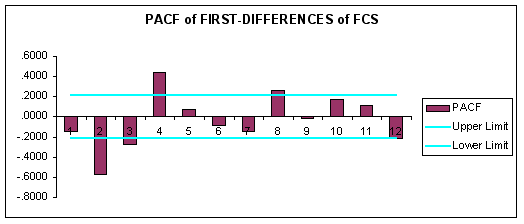
Question #3: Based upon the ACF and PACF of the first-differenced data, what is a candidate Box-Jenkins model?
ANSWER:
To examine this possibility, we generated the following ACF and PACF for the first-differenced data transformed again using first-order seasonal differencing.
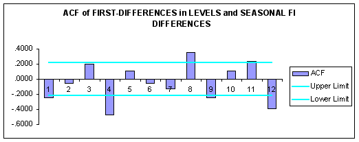
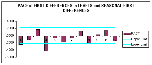
Question #4: Based upon the ACF and PACF of the first-differenced data with first-order seasonal differencing, what is a candidate Box-Jenkins model?
ANSWER:
Accordingly, we generated ACF and PACF correlograms for the first-differenced data with second-order seasonal differencing as reported below.
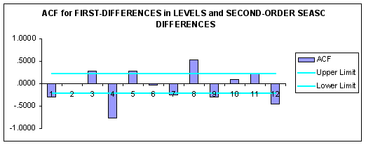
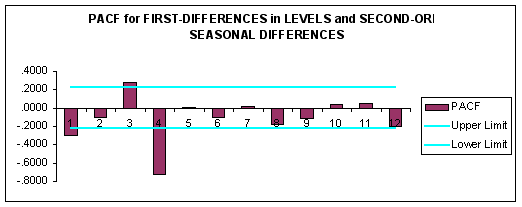
Question #5: Based upon the ACF and PACF for the data transformed by first differences in levels and second seasonal differences, what is a candidate ARIMA model?
ANSWER:
Note: Throughout this case we left the seasonality box blank in the Data Capture screen, which lets FORECASSTXTM diagnose the degree of seasonality in the data. Students who select 4 will obtain slightly different results.
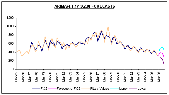
ARIMA(4,1,4)*(0,2,0) forecasts and holdout period results are reported below.
|
Forecast -- Box Jenkins Selected |
|
|
|
||
|
|
Forecast |
|
95% - 5% |
95% - 5% |
|
|
Date |
Quarterly |
Annual |
|
Upper |
Lower |
|
Mar-1996 |
342.85 |
424.88 |
260.83 |
||
|
Jun-1996 |
381.00 |
497.00 |
264.99 |
||
|
Sep-1996 |
377.41 |
519.49 |
235.34 |
||
|
Dec-1996 |
282.23 |
1,383.50 |
|
446.29 |
118.18 |
|
Avg |
345.87 |
1,383.50 |
471.92 |
219.83 |
|
|
Max |
381.00 |
1,383.50 |
519.49 |
264.99 |
|
|
Min |
282.23 |
1,383.50 |
|
424.88 |
118.18 |
|
Audit Trail -- Out of Sample Table (Box Jenkins Selected) |
|
|
|||
|
Original |
Fitted |
Cumulative |
|||
|
Date |
Data |
Data |
MAD |
MAPE |
SSE |
|
Mar-1995 |
371.10 |
373.91 |
19.67 |
0.05 |
690.95 |
|
Jun-1995 |
425.50 |
441.22 |
25.08 |
0.06 |
815.20 |
|
Sep-1995 |
397.30 |
427.83 |
28.48 |
0.07 |
930.00 |
|
Dec-1995 |
313.50 |
307.79 |
24.21 |
0.06 |
938.96 |
|
Avg |
376.85 |
387.69 |
24.36 |
0.06 |
843.78 |
|
Max |
425.50 |
441.22 |
28.48 |
0.07 |
938.96 |
|
Min |
313.50 |
307.79 |
19.67 |
0.05 |
690.95 |
|
StDev |
47.72 |
60.69 |
3.63 |
0.01 |
116.43 |
|
Var |
2,277.10 |
3,683.64 |
13.18 |
0.00 |
13,555.63 |
|
Median |
384.20 |
400.87 |
24.65 |
0.06 |
872.60 |
|
Method Statistics |
|
Value |
|
|
Method Selected |
Box Jenkins |
||
|
Model Selected |
ARIMA(4,1,4) * (0,2,0) |
||
|
T-Test For Non Seasonal AR |
1.01 |
||
|
T-Test For Non Seasonal AR |
0.23 |
||
|
T-Test For Non Seasonal AR |
-0.12 |
||
|
T-Test For Non Seasonal AR |
-10.13 |
||
|
T-Test For Non Seasonal MA |
3.27 |
||
|
T-Test For Non Seasonal MA |
0.36 |
||
|
T-Test For Non Seasonal MA |
0.08 |
||
|
T-Test For Non Seasonal MA |
3.53 |
||
The following accuracy measures are for the holdout period 1995:
|
Accuracy Measures |
|
Value |
|
|
AIC |
928.35 |
||
|
BIC |
947.80 |
||
|
Mean Absolute Percentage Error (MAPE) |
6.63% |
||
|
Sum Squared Error (SSE) |
256,334.81 |
||
|
R-Square |
82.57% |
||
|
Adjusted R-Square |
80.96% |
||
|
Root Mean Square Error |
55.24 |
||
Finally, the ACF and PACF for the ARIMA(4,1,4)*(0,2,0) model residuals are reported below.
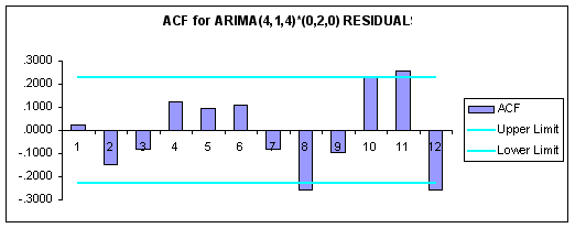
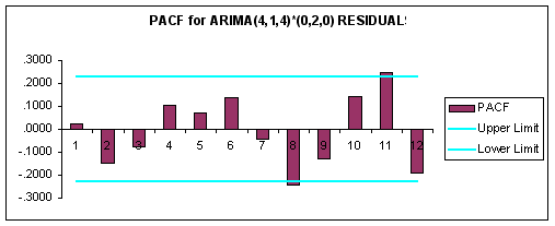
Question #6: Based upon the summary statistics and the ACF and PACF of the ARIMA(4,1,4)*(0,2,0) residuals, evaluate the quality of this model.
ANSWER:
Estimating Box-Jenkins Models using FORECASTTM Expert Selection
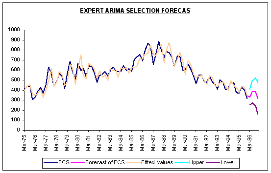
As an alternative to our analysis above, we re-estimated the model using the Expert Selection features of FORECASTXTM. Specifically, we let the software deal with trend and seasonality by the appropriate data transformation and model type. Specifically, we left blank the edit parameters box in the forecast selection screen. The results are reported below.
|
Forecast -- Box Jenkins Selected |
|
|
|
||
|
|
Forecast |
|
95% - 5% |
95% - 5% |
|
|
Date |
Quarterly |
Annual |
|
Upper |
Lower |
|
Mar-1996 |
330.29 |
408.57 |
252.00 |
||
|
Jun-1996 |
384.28 |
494.99 |
273.56 |
||
|
Sep-1996 |
382.02 |
517.62 |
246.43 |
||
|
Dec-1996 |
317.58 |
1,414.17 |
|
474.16 |
161.01 |
|
Avg |
353.54 |
1,414.17 |
473.83 |
233.25 |
|
|
Max |
384.28 |
1,414.17 |
517.62 |
273.56 |
|
|
Min |
317.58 |
1,414.17 |
|
408.57 |
161.01 |
|
Audit Trail -- Out of Sample Table (Box Jenkins Selected) |
|
|
|||
|
Original |
Fitted |
Cumulative |
|||
|
Date |
Data |
Data |
MAD |
MAPE |
SSE |
|
Mar-1995 |
371.10 |
377.39 |
26.03 |
0.07 |
879.88 |
|
Jun-1995 |
425.50 |
435.93 |
32.84 |
0.09 |
1,173.15 |
|
Sep-1995 |
397.30 |
427.95 |
36.82 |
0.10 |
1,404.91 |
|
Dec-1995 |
313.50 |
343.83 |
46.15 |
0.13 |
1,751.30 |
|
Avg |
376.85 |
396.28 |
35.46 |
0.10 |
1,302.31 |
|
Max |
425.50 |
435.93 |
46.15 |
0.13 |
1,751.30 |
|
Min |
313.50 |
343.83 |
26.03 |
0.07 |
879.88 |
|
StDev |
47.72 |
43.52 |
8.41 |
0.02 |
368.44 |
|
Var |
2,277.10 |
1,894.38 |
70.65 |
0.00 |
135,751.00 |
|
Median |
384.20 |
402.67 |
34.83 |
0.10 |
1,289.03 |
As reported below, the Expert Selection feature of FORECASTXTM selects an ARIMA(1,0,0)*(2,0,0) model. This model employs a single non-seasonal AR term along with two seasonal AR terms. Note the model employs no level or seasonal differencing, contrary to our initial ARIMA(4,1,4)*(0,2,0) model.
|
Method Statistics |
|
Value |
|
|
Method Selected |
Box Jenkins |
||
|
Model Selected |
ARIMA(1,0,0) * (2,0,0) |
||
|
T-Test For Non Seasonal AR |
8.98 |
||
|
T-Test For Seasonal AR |
4.29 |
||
|
T-Test For Seasonal AR |
3.18 |
||
|
T-Test For Constant |
0.19 |
||
The following accuracy statistics relate to the holdout period 1985Q1-1985Q4.
|
Accuracy Measures |
|
Value |
|
|
AIC |
898.73 |
||
|
BIC |
908.45 |
||
|
Mean Absolute Percentage Error (MAPE) |
6.69% |
||
|
Sum Squared Error (SSE) |
198,168.68 |
||
|
R-Square |
86.52% |
||
|
Adjusted R-Square |
86.02% |
||
|
Root Mean Square Error |
48.57 |
||
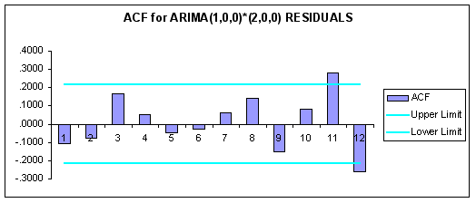
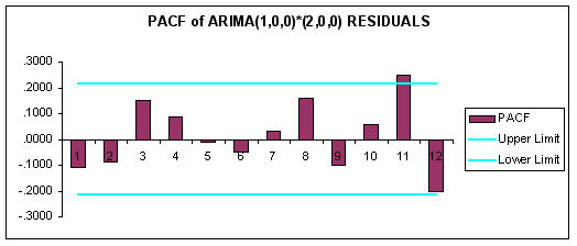
Finally, we estimated the following correlograms for the ARIMA(1,0,0)*(2,0,0) model residuals.
We also generated the following summary statistics for the ARIMA(1,0,0)*(2,0,0) residuals:
|
Forecast Statistics |
Value |
|
|
Durbin Watson |
2.23 |
|
|
Ljung-Box |
1.19 |
|
Here the Ljung-Box-Pierce Q statistics has a chi-square distribution with 84 — 3 = 81 degrees of freedom. The 5% critical value for 30 degrees of freedom is 43.773. Accordingly, since our reported Ljung-Box value is less than this we cannot reject the null of a white noise series in the ARIMA(1,0,0)*(0,2,0) residuals. Accordingly, the ARIMA(1,0,0)*(0,2,0) model is a candidate forecasting model for FCS. But how well does the model perform relative to others?
Comparing Models
Question #7: Contrast and compare the ARIMA models with the decomposition models of Chapter Six, Case #2. Which model has the better out-of-sample accuracy over the holdout period?
ANSWER:
Student Practice Question
Question #1: Redo this assignment using domestic car sales as the dependent variable. Specifically, compare and contrast Box-Jenkins and Time Series Decomposition forecasts of domestic car sales data (See C6_Case2.xls). Compare and contrast your results with those of this case.