Goal: This utilizes two univariate time-series models to produce forecasts and examines whether different ways to model the same information justify the efforts involved in forecast combination.

Specifically, this case examines:

• Dealing with Seasonal Data using FORECASTX^TM
• Testing Conditions for Forecast Combination to be Effective
• Estimating Optimal Weights in the Forecast Combination Process
• Comparing fit of Combination versus Individual Forecasts.

The spreadsheet for this problem is C8_Case2.xls. It contains revenue passenger miles (RPM) data for airline travel.

Data on international revenue-passenger miles (RPM) is published monthly by the U.S. Department of Transportation. (Recall this data was analyzed in Problem #3 in this chapter).

Our goal is to examine improvement in model fit using forecast combination over the sample period.

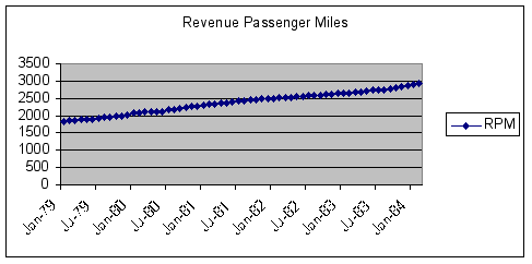
To examine graphically any trend or seasonality in the data, we generated a time-series plot of the RPM data.

Question #1: Based on examination of the time-series plot of RPM, does the data exhibit significant trend or seasonality?

ANSWER:

To further analyze the data for seasonality, generate ACF and PACF correlograms reported below.

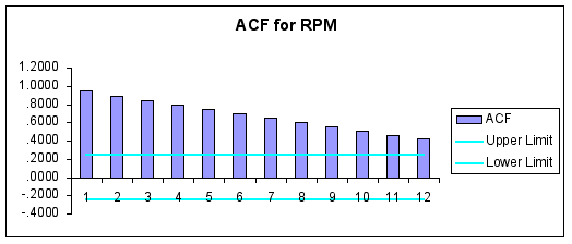
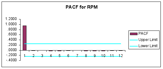
Question #2: Are the data stationary? Explain.

ANSWER:

Accordingly, for this case we have seasonal data with a trend. To handle these complications requires some form of data transformation and/or modeling of seasonality and trend. To accomplish this we shall employ the Expert Selection aspects of FORECASTX^TM, and then combine forecasts.

Using FORECASTX^TM, we first developed a Box-Jenkins model using historical data with no holdback or forecast period designated.

Estimation results are presented below.

Note that FORECASTX^TM chooses an ARIMA(0,1,0)*(1,0,0) model as optimal.

In-sample accuracy statistics are reported below.

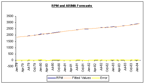
Question #3: How well does our ARIMA(0,1,0)*(1,0,0) model fit the data?

ANSWER:

An alternative way of forecasting RPM is Winter’s smoothing which handles trend and seasonality.

Estimation results using Winter’s smoothing are reported below.

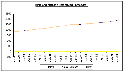
Question #4: How well does the Winter’s model fit the data?

ANSWER:

Question #5: Can you make the case that these two methods should be combined to generate forecasts?

ANSWER:

To examine whether forecast combination is possible, we estimate the following regression over the sample period.

Question #6: Can the two models be combined to generate unbiased forecasts? Explain.

ANSWER:

Next, calculate the optimal weights to be given to each method by estimating the following regression:

In-sample fit statistics are reported below.

An in-sample plot of RPM and combined model forecasts is reported below.

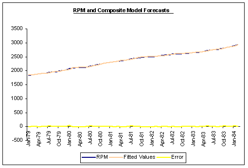
Question #7: Report the optimal weights below. Explain!

ANSWER:

In-sample RMSE for a three models is reported below.

Question #8: Based upon the combined forecasts results reported above, are there benefits to combining these two forecasting models?

ANSWER:

Question #1: Redo this case with another variable that is highly seasonal. Contrast and compare your results with those of this case.