We encounter many problems analyzing these data by regression because some predictor variables are highly correlated. For example, Ex0 and Ex1, which measure police expenditures in consecutive years, have a correlation of .99. Wealth (W) and income inequality (X) are also highly correlated, as are U1 and U2, which measure unemployment in two different age groups. When predictor variables are highly correlated, the model is said to be nearly collinear. The result is that our estimated coefficients are unstable; removing one variable from the model may cause the results for the other variables to change dramatically.

In addition, the causal relationship between Ex0 (expenditures in 1960) and crime rate is unclear. Do increased expenditures affect the crime rate, or does the crime rate motivate an increase in expenditures?

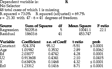
In one possible analysis, predictors are removed from the model until only the 5% significant predictors Age, Ed, U2, X, and Ex0 remain. The results of this model are in Figure 1. This model demonstrates that it is important to look at the direction of the coefficients. From these coefficients, it appears that more education and police expenditures increase the crime rate. Perhaps there is another variable, a "lurking variable" not collected with these data, which causes both education and crime rate to increase together.

This data set is a good example of what can go wrong in a regression analysis.