First, we consider Internal Reflection. The light is incident from a dense medium such as water with index of refraction n₁ and passes into a less dense medium with index of refraction n₂ < n₁. In this case, Snell's law limits the possible incident angles for refraction to theta < arcsin(n₂/n₁). This is called the angle of total reflection. Beyond this angle, all incident light is reflected!

> n_1 := 3/2;

> n_2 := 1;

> phi := theta*Pi/180;

> xi := arcsin(n_1*sin(phi)/n_2);

> Theta_max := 180*arcsin(n_2/n_1)/Pi;

> R_perp:= (sin(xi-phi)/sin(xi+phi))^2;

> R_para:= (tan(xi-phi)/tan(xi+phi))^2;

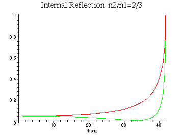
> plot({R_perp,R_para},theta=0..Theta_max,title="Internal Reflection n2/n1=2/3");

In green, we plot the reflection coefficient for parallel polarization and in red, we plot the coefficient for perpendicular polarization. The angle at which R_|| = 0 is called Brewster's angle. Note that both coefficients = 1 at the angle of total reflection.

Next, we consider light incident from a less dense medium such as air with index of refraction n₁ passing into a dense medium such as glass with index of refraction n₂ > n₁.

> n_1 := 1;

> n_2 := 3/2;

> phi := theta*Pi/180;

> xi := arcsin(n_1*sin(phi)/n_2);

> R_perp:= (sin(xi-phi)/sin(xi+phi))^2;

>

> R_para:= (tan(xi-phi)/tan(xi+phi))^2;

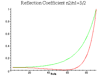
> plot({R_perp,R_para},theta=0..90,title="Reflection Coefficient n2/n1=3/2");

In green, we plot the reflection coefficient for perpendicular polarization and in red, we plot the coefficient for parallel polarization. Again, the angle at which R_|| = 0 is called Brewster's angle. Note that both coefficients = 1 at 90 degrees. Does it surprise you that in both examples the two reflection coefficients = 0.04 when theta=0?

Now, let's look at the amplitudes. First we consider parallel incidence:

> Er_para := tan(xi-phi)/tan(xi+phi);

> Et_para := n_1*(1-Er_para)/n_2;

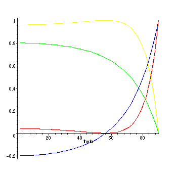
> plot({Er_para,Et_para,R_para,1-R_para},theta=0..90);

The blue curve is the relative amplitude of the reflected wave, the green curve is the relative amplitude of the transmitted wave, the red curve is the reflection coefficient, and the yellow curve is the transmission coefficient. All of these are for parallel incidence.

Finally, we consider amplitudes for perpendicular incidence:

> Er_perp := sin(xi-phi)/sin(xi+phi);

> Et_perp := 1+Er_perp;

>

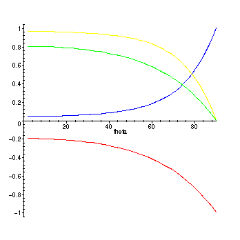
> plot({Er_perp,Et_perp,R_perp,1-R_perp},theta=0..90);

The red curve is the relative amplitude of the reflected wave, the green curve is the relative amplitude of the transmitted wave, the blue curve is the reflection coefficient, and the yellow curve is the transmission coefficient. All of these are for perpendicular incidence.