Chapter 13, Table 12: Testing Polynomial Contrasts via SPSS point and click

For the hypothetical data contained in Table 13.2, the linear and quadratic D variables were formed by making use of the appropriate coefficients from Appendix Table A.10. Because the eight participants were measured at three occasions, both a linear and a quadratic effect can be tested. The question of interest in this instance is: “Is there a linear and/or quadratic trend exhibited by the group over time?” Recall that in the book (pages 646-647) it was shown that the D variables for linear and quadratic effects led to an omnibus F test of 19.148, which was a value previously obtained for the omnibus effect. Because the particular values chosen for the D variables do not matter (unless it leads to a linear combination of columns), we will focus only on the tests of the individual contrasts when analyzing the data given in Table 12.

Because columns one and two already represent the linear and quadratic effect respectively, all that needs to be done is to test mean of the column in order to determine if it differs from zero. The easiest way to do this is by clicking Analyze, and then, after moving to the Compare Means menu, clicking One-Sample T Test. Each of the effects (linear and quadratic) needs to be done individually. This is done by moving the column representing the effect of interest, we first analyze the linear trend, by moving it into the Test Variable(s) box. Note that the Test Value should be zero (which it is by default).

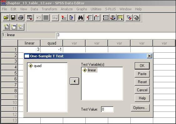
After moving the linear trend to the Test Variable(s) box, clicking OK will produce the answer given on page 648. Note that the results from SPSS produce a t value. The results given in the text are in terms of F. Squaring the t value of 3.969 will yield the F value of 15.75 given on page 648.

Follow the same procedure for the quadratic effect will produce the test of the quadratic effect, as illustrated below:

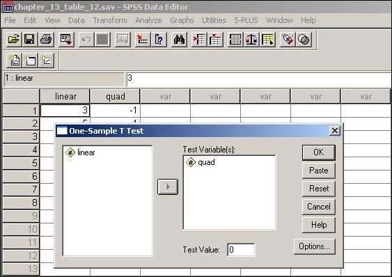
After moving the quadratic particular trend to the Test Variable(s) box, clicking OK will produce the results.

Note that a more direct way to carryout tests of polynomial trends is to specify polynomial contrasts from within the Repeated Measures menu. When defining the levels of the repeated factor (as we did early in this chapter), the Contrasts button can be clicked (bottom left-hand side of the dialog box) and then Polynomial specified. This requires directly inputting the raw data (rather than the linear composite from making use of the coefficients in Appendix Table A. 10).