Evaluating Double Integrals
Nancy K. Stanton
based on original versions © 2000-2005 by Paul Green and Jonathan Rosenberg, modified with permission
Contents
Evaluating Iterated Integrals
Evaluating a multiple integral involves expressing it as an iterated integral, which can then be evaluated either symbolically or numerically. We begin by discussing the evaluation of iterated integrals.
Example 1
We evaluate the iterated integral
To evaluate the integral symbolically, we can proceed in two stages.
syms x y
firstint=int(x*y,y,1-x,1-x^2)
answer=int(firstint,x,0,1)
firstint =

(x^2*(x - 1)^2*(x + 2))/2


answer =

1/24
We can even perform the two integrations in a single step:
int(int(x*y,y,1-x,1-x^2),x,0,1)
ans =

1/24
There is, of course, no need to evaluate such a simple integral numerically. However, if we change the integrand to, say, exp(x^2 - y^2), then MATLAB will be unable to evaluate the integral symbolically, although it can express the result of the first integration in terms of erf(x), which is the (renormalized) antiderivative of exp(-x^2).
int(int(exp(x^2-y^2),y,1-x,1-x^2),x,0,1)
Warning: Explicit integral could not be found.

ans =

int((pi^(1/2)*exp(x^2)*(erf(x - 1) - erf(x^2 - 1)))/2, x = 0..1)
However, we can evaluate the integral numerically, using double.
double(int(int(exp(x^2-y^2),y,1-x,1-x^2),x,0,1))
Warning: Explicit integral could not be found.

ans =

    0.1675
Problem 1
Evaluate the iterated integrals
and
Finding the Limits
We will now address the problem of determining limits for a double integral from a geometric description of the region of integration. While MATLAB cannot do that for us, it can provide some guidance through its graphics and can also confirm that the limits we have chosen define the region we intended. For a first example, we will consider the bounded region between the curves y = 2x+2 and y = exp(x). We begin by plotting the two curves on the same axes. You may need to experiment with the interval to get a useful plot; it should be large enough to show the region of interest, but small enough so that the region of interest occupies most of the plot.
y1=exp(x);y2=2*x+2;
ezplot(y1,[-1,2]); hold on;
ezplot(y2,[-1,2]); hold off;
title('region bounded by y = 2x+2 and y = e^x')
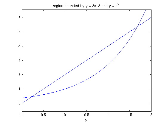
We can see from the plot that, to define the bounded region between the two graphs, exp(x) should be the lower limit for y, and 2x+2 should be the upper limit. In order to find the limits for x, we need the values for which the two functions coincide. We use solve to find them.
solve(y1-y2)
ans =

- lambertw(0, -1/2*exp(-1)) - 1
Hmm..., not clear what this means, but we can convert to a numerical value:
lim1=double(ans)
lim1 =

   -0.7680
For the other solution, we use fzero:
lim2=fzero(char(y1-y2),2)
lim2 =

    1.6783
Now that we have found the limits, we can use the following M-file verticalRegion to visualize the region they define so that we can check that it is the same as the region we had in mind. This program plots the two curves in two different colors: red for the function entered first, and blue for the function entered second, and shades the region in between in cyan.
type verticalRegion
function out = verticalRegion(a, b, f, g)
%VERTICALREGION is a version for Matlab of the routine on page 157
%  of "Multivariable Calculus and Mathematica" for viewing the region
%  bounded by two curves. f and g must be names of functions;
%  a and b are the limits.  The function f is plotted in red and the
%  function g in blue, and lines are drawn connecting the two curves
%  to illustrate the region they bound. The function g must have a variable
%  in it, so if it's supposed to be a constant, try a fudge like
%  '0 + eps*x'.
var=findsym(g);
a=double(a);b=double(b);
%This guarantees these are floating point
% numbers and not just symbolic expressions like sqrt(2)
xx=a:(b-a)/40:b;
fin=inline([vectorize(f+var-var),'+zeros(size(',char(var),'))'],char(var));
gin=inline(vectorize(g+var-var),char(var));
plot(xx,fin(xx),'r');
hold on
plot(xx,gin(xx),'b');
for xxx=a:(b-a)/20:b,
 Y=[fin(xxx), gin(xxx)];
 plot([xxx, xxx], Y, 'c');
end
title(['region between ',char(f),' and ',char(g)])
hold off
verticalRegion(lim1,lim2,y1,y2)
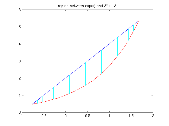
Evidently our limits define the right region. We can now use them to integrate any function we like over the region in question. To find the area of the region, for example, we integrate the function 1. Since our limits for x are numerical, a symbolic calculation is not of much use directly, so we use double to convert to a numerical answer.
area=double(int(int(1,y1,y2),lim1,lim2))
area =

    2.2270
Of course, the area between two curves could just as easily have been evaluated as the integral of the difference between the two functions of x whose graphs define the region; that is to say the first integration in this case is so simple that one can write down the result as easily as the integral. However, we can also integrate any function we like over the same region, changing only the integrand. For instance:
newint=double(int(int(sin(x^2+y^2),y,y1,y2),x,lim1,lim2))
Warning: Explicit integral could not be found.

newint =

    0.2892
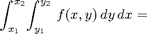
MATLAB has its a double integrator, called dblquad. There is a complication in using dblquad; it does not accept variable limits. In order to use dblquad, we must make a change of variables in the inner integral. Fortunately, it is always the same one. We set y=y1+u(y2-y1) so that as u varies from 0 to 1, y varies from y1 to y2, and then integrate over x and u instead of over x and y. Note that dy=(y2-y1)du. This gives the identity
dblquad demands a vectorized function (not symbolic expression) as an input. All this is easily implemented. We illustrate it in the example above, so we are integrating  . Our change of variables becomes
  and
and  so the new integrand is
g = @(x,y) sin(x.^2+y.^2);
h = @(x,u) g(x, exp(x)+u*(2*x+2-exp(x))).*(2*x+2-exp(x))
newint2=dblquad(h,lim1,lim2,0,1)
newint-newint2
h =

    @(x,u)g(x,exp(x)+u*(2*x+2-exp(x))).*(2*x+2-exp(x))


newint2 =

    0.2892


ans =

  -2.2080e-07
The answers provided by these two distinct methods agree to seven decimal places.
Because of the syntactical complications of using dblquad on a region that is not rectangular, Jonathan Rosenberg and his colleagues created M-files symint2 and numint2, which have identical calling syntax and implement, respectively, symbolic double integration using int, and numerical double integration using dblquad. The advantage of the identical syntax is that if symint2 fails, one can try numint2 instead with a minimum of editing. We illustrate them by repeating the two previous computations.
type symint2
function out=symint2(integrand,var1,varlim1,varlim2,var2,lim1,lim2)
%SYMINT2 Symbolically evaluate double integral.
%   NUMINT2 is basically a "wrapper" for iterated application of INT.
%   The INNER integral should be written first.
%   Example:
%       syms x y
%       symint2(x,y,0,x,x,1,2) integrates
%       the function x over the trapezoid 1<x<2, 0<y<x,
%       and gives the symbolic output 7/3.
%   See also NUMINT2.
out=int(int(integrand,char(var1),varlim1,varlim2),char(var2),lim1,lim2);
type numint2
function out=numint2(integrand,var1,varlim1,varlim2,var2,lim1,lim2)
%NUMINT2 Numerically evaluate double integral.
%   NUMINT2 is basically a "wrapper" for DBLQUAD, to
%   get around the fact that the latter is only designed for integration
%   over a rectangle, and requires inline vectorized input.  The
%   INNER integral should be written first.
%   Example:
%       syms x y
%       numint2(x,y,0,x,x,1,2) integrates
%       the function x over the trapezoid 1<x<2, 0<y<x,
%       and gives the numerical output 2.3333.
%   See also SYMINT2.
syms uU
newvar1=varlim1+uU*(varlim2-varlim1);
integrand2=subs(integrand,var1,newvar1)*(varlim2-varlim1);
integrand3=inline([char(vectorize(integrand2)),'.*ones(size(uU))'],'uU',char(var2));
out=dblquad(integrand3,0,1,lim1,lim2);
double(symint2(sin(x^2+y^2),y,y1,y2,x,lim1,lim2))
numint2(sin(x^2+y^2),y,y1,y2,x,lim1,lim2)
Warning: Explicit integral could not be found.

ans =

    0.2892


ans =

    0.2892
numint2 requires outer limits which MATLAB views as numerical, so you might have to apply the command double to your outer limits before using numint2.
Note: In some problems, dblquad and numint2 do not work that well, and spit out long lists of warning messages. In next week's lesson, we will discuss another package called nit, or "numerical integration toolbox", that usually corrects the problem.
Problem 2
Let R be the region bounded by the curves y=3*x^2 and y=2*x+3.
a) Determine the limits of integration for a double integral over R; confirm your limits by using verticalRegion.
b) Evaluate
both using double and int (or double and symint2), and using dblquad (or numint2).
Integrating over Implicitly Defined Regions
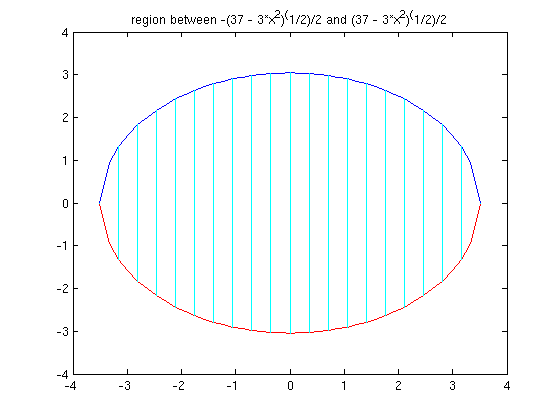
Let us now turn to the process of integrating over a region bounded by a level curve of a function of two variables. Once again, the real issue is the determination of the limits of integration. We will consider the region bounded by the ellipse 3*x^2+4*y^2=37. Although it is not strictly necessary in this case, we will begin by plotting the ellipse.
ezplot(3*x^2+4*y^2-37, [-4, 4, -4, 4]), axis equal
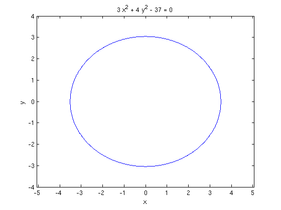
We can see from the plot that this region is vertically simple. We obtain our y limits by solving the equation of the ellipse for y in terms of x.
ylims=solve(3*x^2+4*y^2-37,y)
ylims =

 -(37 - 3*x^2)^(1/2)/2
  (37 - 3*x^2)^(1/2)/2
The two solutions give the upper and lower limits for y. We can find the limits for x by setting their difference to 0 and solving for x.
y1=ylims(1)
y2=ylims(2)
xlims=solve(y1-y2,x)
x1=xlims(2)
x2=xlims(1)
y1 =

-(37 - 3*x^2)^(1/2)/2


y2 =

(37 - 3*x^2)^(1/2)/2


xlims =

  (3^(1/2)*37^(1/2))/3
 -(3^(1/2)*37^(1/2))/3


x1 =

-(3^(1/2)*37^(1/2))/3


x2 =

(3^(1/2)*37^(1/2))/3
We can confirm our limits, using verticalRegion. The first two arguments to verticalRegion must be numerical, rather than symbolic. Therefore, we must apply double to x1 and x2.
verticalRegion(double(x1),double(x2),y1,y2)
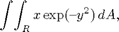
We can now integrate any function we desire over the region bounded by the ellipse.
Problem 3
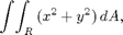
Integrate

a) Over the region bounded by the ellipse 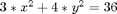 .
.
b) Over the region bounded by the curve  .
.
Polar Coordinates
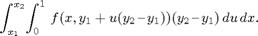
We conclude this lesson with a discussion of integration in polar coordinates. We consider integrating the function  over the disk bounded by the circle
  We begin by expressing the function whose vanishing defines the boundary curve in polar coordinates.
syms r th
polarfun=simplify(subs((x-1)^2+y^2-1, [x,y],[r*cos(th),r*sin(th)]))
polarfun =

r^2 - 2*r*cos(th)
Next we solve the equation of the boundary curve for r in terms of theta, to obtain the limits for r.
rlims=solve(polarfun,r)
rlims =

         0
 2*cos(th)
Since the disk we are interested in lies entirely to the right of the x-axis, the appropriate limits for theta are  and
and  . Bearing in mind that we must include a factor of r when integrating in polar coordinates, we can now set up and evaluate an iterated integral in any of the usual ways. For example:
double(int(int(r*exp(-r^2),0,2*cos(th)),-pi,pi))
Warning: Explicit integral could not be found.

ans =

    2.1724
Problem 4
Reevaluate the integral above using numint2.
Additional Problems
1. Evaluate
where R is the triangle with vertices at (0,0), (0,2) and (3,0). Hint: begin by determining the equation of the oblique side of the triangle. Use verticalRegion to confirm your limits.
2. Evaluate
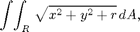
where R is the region bounded by the cardioid

3. Compute the area of the region bounded by the two curves  and
and  .
.