Visualizing Functions of Several Variables and Surfaces
Nancy K. Stanton
based on original versions © 2000-2005 by Paul Green and Jonathan Rosenberg, modified with permission
Contents
Functions of Two Variables
A function f of two variables is a rule which takes two numerical inputs, say x and y, and produces a numerical output, written f(x,y). Sometimes it will be preferable to think of f as taking one (2-dimensional) vector input instead of two scalar inputs. There are two main ways to visualize such a function:
- a contour plot, or a two-dimensional picture of the level curves of the surface, which have equations of the form f(x,y) = c, where c is a constant;
- the graph of the function, which is the set of points (x,y,z) in three-dimensional space satisfying f(x,y) = z.
We begin by illustrating how to produce these two kinds of pictures in MATLAB, using MATLAB's easy-to-use plotting commands, ezcontour and ezsurf. We take f sufficiently complicated to be of some interest. Note that our plotting commands can take as input an expression that defines a function, rather than a function itself. (In other words, it is not necessary to use an M-file or an anonymous function as an input to the plotting command.)
syms x y
f=((x^2-1)+(y^2-4)+(x^2-1)*(y^2-4))/(x^2+y^2+1)^2
f =

((x^2 - 1)*(y^2 - 4) + x^2 + y^2 - 5)/(x^2 + y^2 + 1)^2
We start with the contour plot. The only arguments we use in ezcontour are the expression, whose contours are to be plotted, and the ranges of values for x and y.
ezcontour(f, [-3, 3, -3, 3])
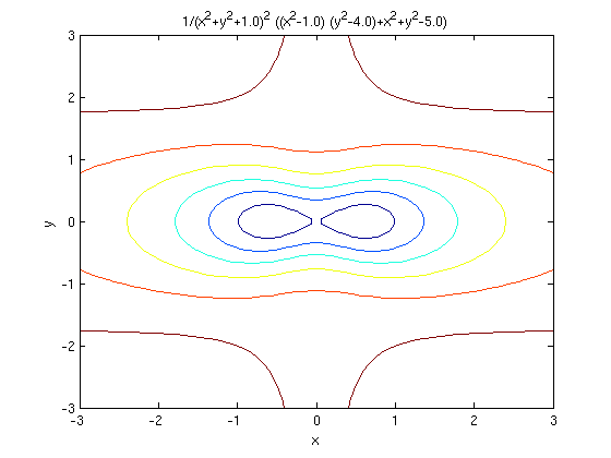
The color coding in the contour plot tells us how the values of the constant c are varying. One of the level curves in this case is misleading; the contour in dark blue in the middle should be a figure-eight. We will see in the next lesson why this is so and how to detect it.
Now for a picture of the graph of f:
ezsurf(f, [-3, 3, -3, 3])
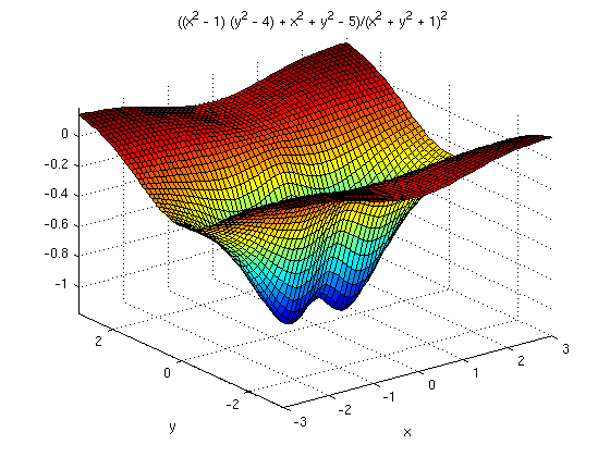
Once you execute this command, you can rotate the figure in space to be able to view it from different angles. Note that the graph is a surface, in other words, a two-dimensional geometric object sitting in three-space. Every graph of a function of two variables is a surface, but some surfaces are not graphs. Note that MATLAB again color-codes the output, with blue denoting the smallest values of the function, and red denoting the largest.
Finer Points of Plotting with MATLAB
We begin with a brief discussion of how MATLAB does its plotting. The arguments to a MATLAB [non-ez] plotting function, such as surf, plot, plot3, mesh, or contour, are two or three identically shaped arrays. The positions in these arrays correspond to parameter or coordinate values; the entries give the coordinates as functions of the parameters (which may be identical with the coordinates). Thus for a curve, the arguments are usually linear arrays, or vectors, while for a surface, they are rectangular arrays, or matrices.
We will illustrate how this works to plot the graph of the function f above. In this case, the parameters are also the x and y coordinates. We start by defining the coordinate grid with the meshgrid command.
[X1,Y1]= meshgrid(-5:.2:5,-5:.2:5);
We use X1 and Y1, rather than x and y, because we want to reserve the latter for symbolic variables. The command creates a grid with both the x and y coordinates varying in steps of .2 from -5 to 5. Note the use of the semicolon! If we had not suppressed the output, MATLAB would have printed out the entire grid.
Next, we must turn f into a vectorized function, since it must operate on our arrays of x- and y-values. Then we evaluate this function at each point of the grid, to define the array of z-coordinates for the plot.
zfun = @(x, y) eval(vectorize(f))
Z1=zfun(X1,Y1);
zfun =

    @(x,y)eval(vectorize(f))
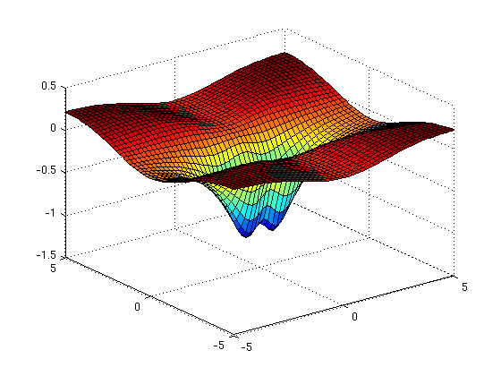
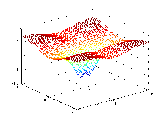
We can now proceed with the plot in any of several ways:
surf(X1,Y1,Z1)
mesh(X1,Y1,Z1)
plot3(X1,Y1,Z1)
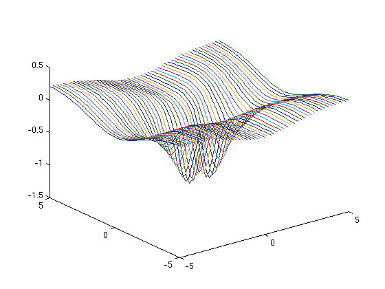
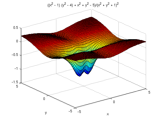
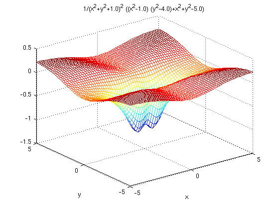
By now, it may have occurred to you that we could have issued exactly the same sequence of commands for any parametrized surface. The essential information for such a plot is the name of the symbolic vector that defined the parametrization, the specification of the parameter grid, and the plotting function to be used. We could have also used the ez plotting functions, as in:
ezsurf(f,[-5,5,-5,5])
ezmesh(f,[-5,5,-5,5])
Problem 1
- (a) By using the step by step procedure followed above obtain surface, mesh and line plots of the function

- (b) Obtain surface and mesh plots by using ezsurf and ezmesh.
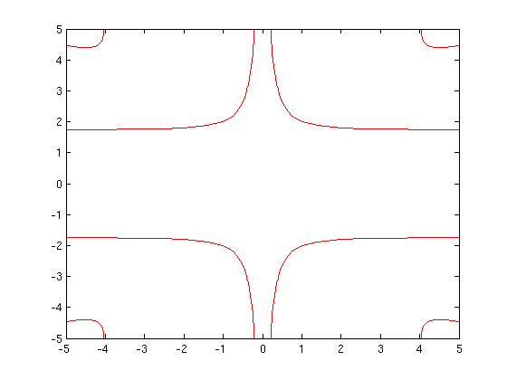
Now let's go back to contour plots. ezcontour does not allow us to specify how many or which contours we want, or the colors of the contours. However, we can accomplish this using contour. For instance, we can plot the level curves f = 0 and f = 0.2 in red by typing:
contour(X1, Y1, Z1, [0,.2], 'r')
Problem 2
(a) Obtain a contour plot of the function g(x,y) defined in Problem 1 using MATLAB's default contours.
(b) Superimpose on the a plot of part (a) a plot showing the contours g(x,y) = 0, g(x,y)= 0.2, and g(x,y) = 0.4 in red.
Surfaces
Although we will analyze the function f(x,y) further in the next lesson, we abandon it for the present. Instead we discuss how to plot a surface that is not the graph of a function of two variables, such as a sphere. There are two main techniques available:
- (1) We can write the surface as a level surface f(x,y,z) = c of a function of three variables, f(x,y,z).
- (2) We can parameterize the surface by writing x, y, and z each as functions of two parameters, say s and t. This is analogous to parameterizing a curve and writing x, y, and z each as a function of t.
We begin with the first technique. The graph of a function of three variables would require a four dimensional plot, which is beyond MATLAB's capabilities, but we can draw a picture of a single level surface of the function. This can be viewed as a three dimensional version of contour plotting. A plot showing more than one level surface is usually difficult to interpret, so we will discuss plotting a single level surface. For this one can use the following M-file implicitplot3d:
type implicitplot3d.m
function out=implicitplot3d(varargin)
%IMPLICITPLOT3D 3-D implicit plot
% IMPLICITPLOT3D(eq, val, xvar, yvar, zvar, xmin, xmax,
% ymin, ymax, zmin, zmax) plots an implicit equation
% eq=val, where eq is either symbolic expression of (symbolic)
% variables xvar, yvar, and zvar in the indicated ranges, or
% a string representing such an expression, and val is a number.
% If xvar, yvar, and zvar are not specified, it is assumed they are
% x, y, z in the symbolic case, or 'x', 'y',and 'z' in the
% string form of the command, respectively.
% The optional parameter plotpoints (added at the end)
% gives the number of steps in each direction between plotting points.
%
% Example: implicitplot3d('x^2+y^2+z^2', 5, -3, 3, -3, 3, -3, 3)
% plots the sphere 'x^2+y^2+z^2=5' with 'x', 'y', and 'z'
% going from -3 to 3.
% implicitplot3d('x^2+y^2+z^2', 5, -3, 3, -3, 3, -3, 3, 30)
% does the same with higher accuracy.
% written by Jonathan Rosenberg, 7/30/99
% rewritten for MATLAB 7, 8/22/05

if nargin<8
    error('not enough input arguments -- need at least expression string, value, xmin, xmax, ymin, ymax, zmin, zmax');
end

if nargin==10, error('impossible number of input arguments'); end

if nargin>12, error('too many input arguments'); end

% Default value of plotpoints is 10.
plotpoints=10;

eq=varargin{1}; val=varargin{2};
stringflag=ischar(eq); % This is 'true' in the string case,
% 'false' in the symbolic case.


% Next, handle subcase where variable names are missing.
if nargin<10
  if stringflag  % First we deal with the string case.
      xvar='x'; yvar='y'; zvar='z';
  else % Now deal with the case where eq is symbolic.
      syms x y z; xvar=x; yvar=y; zvar=z;
  end
  xmin=varargin{3}; xmax=varargin{4};
  ymin=varargin{5}; ymax=varargin{6};
  zmin=varargin{7}; zmax=varargin{8};
  if nargin==9, plotpoints=varargin{9}; end
end
% Next, handle subcase where variable names are included.
if nargin>10
  xvar=varargin{3}; yvar=varargin{4}; zvar=varargin{5};
  xmin=varargin{6}; xmax=varargin{7};
  ymin=varargin{8}; ymax=varargin{9};
  zmin=varargin{10}; zmax=varargin{11};
  if nargin==12, plotpoints=varargin{12}; end
end


if stringflag
    F = vectorize(inline(eq,xvar,yvar,zvar));
else
    F = inline(vectorize(eq),char(xvar),char(yvar),char(zvar));
end
[X Y]= meshgrid(xmin:(xmax-xmin)/plotpoints:xmax, ymin:(ymax-ymin)/plotpoints:ymax);

%% Go through zvalues one at a time. For each one, plot corresponding
%% contourplot in x and y, with that z-value.  We could use "contour"
%% except that it makes a "shadow", so we copy some of
%% the code of "contour".

for z=zmin:(zmax-zmin)/plotpoints:zmax
    lims = [min(X(:)),max(X(:)), min(Y(:)),max(Y(:))];
    c = contours(X,Y,F(X,Y,z), [val val]);
    limit = size(c,2);
    i = 1;
    h = [];
	while(i < limit)
	  npoints = c(2,i);
	  nexti = i+npoints+1;
	  xdata = c(1,i+1:i+npoints);
	  ydata = c(2,i+1:i+npoints);
	  zdata = z + 0*xdata;  % Make zdata the same size as xdata
	  line('XData',xdata,'YData',ydata,'ZData',zdata); hold on;
	  i = nexti;
    end
end
view(3)
xlabel(char(xvar))
ylabel(char(yvar))
zlabel(char(zvar))
title([char(eq),' = ',num2str(val)], 'Interpreter','none')
hold off
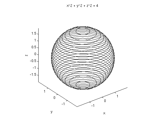
Here's an example:
syms x y z; h=x^2+y^2+z^2; clf; % Clear old figure
implicitplot3d(h, 4, -3, 3, -3, 3, -3, 3, 40); axis equal
Problem 3
Plot the hyperboloid

(Think of it as a level surface.)
Parameterized Surfaces
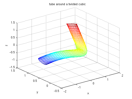
We have now plotted surfaces as graphs of functions of two variables or as level surfaces of functions of three variables. The third technique is (2) above, using a parameterization, which we have already used in a previous lesson. We return to the tube around the twisted cubic which was introduced in Matlab Assignment 3, Curves. Now we only need the parametrization of the tube itself.
syms s t
tctube=[ t- 1/5*cos(s)*t*(2+9*t^2)/(9*t^4+9*t^2+1)^(1/2)/(1+4*t^2+9*t^4)^(1/2)+3/5*sin(s)*t^2/(9*t^4+9*t^2+1)^(1/2),  ...
    t^2-1/5*cos(s)*(-1+9*t^4)/(9*t^4+9*t^2+1)^(1/2)/(1+4*t^2+9*t^4)^(1/2)-3/5*sin(s)*t/(9*t^4+9*t^2+1)^(1/2), ...
    t^3+3/5*cos(s)*t*(1+2*t^2)/(9*t^4+9*t^2+1)^(1/2)/(1+4*t^2+9*t^4)^(1/2)+1/5*sin(s)/(9*t^4+9*t^2+1)^(1/2)]
tctube =

[ t + (3*t^2*sin(s))/(5*(9*t^4 + 9*t^2 + 1)^(1/2)) - (t*cos(s)*(9*t^2 + 2))/(5*(9*t^4 + 4*t^2 + 1)^(1/2)*(9*t^4 + 9*t^2 + 1)^(1/2)), t^2 - (3*t*sin(s))/(5*(9*t^4 + 9*t^2 + 1)^(1/2)) - (cos(s)*(9*t^4 - 1))/(5*(9*t^4 + 4*t^2 + 1)^(1/2)*(9*t^4 + 9*t^2 + 1)^(1/2)), sin(s)/(5*(9*t^4 + 9*t^2 + 1)^(1/2)) + t^3 + (3*t*cos(s)*(2*t^2 + 1))/(5*(9*t^4 + 4*t^2 + 1)^(1/2)*(9*t^4 + 9*t^2 + 1)^(1/2))]
Do not be daunted by the complexity of this expression; we can use ezmesh to recreate the plot of the tube that shows the twisting of the curves of constant s.
ezmesh(tctube(1), tctube(2), tctube(3), [0, 2*pi, -1, 1])
title 'tube around a twisted cubic'
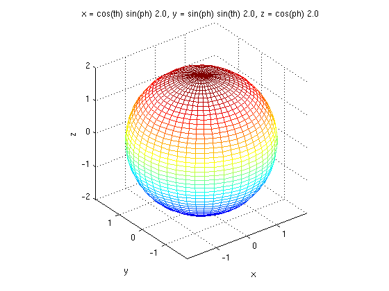
Other surfaces can also be parametrized. In particular, the sphere we plotted as a level surface can also be plotted parametrically (with better results), using spherical coordinates. We use ph and th to represent the angles phi and theta. Note the use of axis equal to make sure our plot looks like a sphere and not just an ellipsoid.
syms ph th
ezmesh(2*sin(ph)*cos(th), 2*sin(ph)*sin(th), ...
    2*cos(ph), [0, pi, 0, 2*pi])
axis equal
Essentially the same parametrization can be used for an ellipsoid by replacing the numerical coefficients of the three components, which were all equal to 2 in the above case of the sphere, by the lengths of the respective semi-major axes.
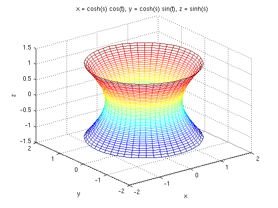
Hyperboloids can be conveniently parametrized using hyperbolic functions. The essential identity to bear in mind is

The following line parametrizes and plots the hyperboloid of one sheet

ezmesh(cosh(s)*cos(t),cosh(s)*sin(t),sinh(s), [-1, 1, 0, 2*pi])
Problem 4
Parametrize and replot parametrically the hyperboloid you plotted in Problem 3.
Additional Problems
1. Plot the hyperboloid of two sheets

(a) As a level surface.
(b) By parametrizing the upper and lower sheets separately and plotting them both in the same figure using hold on.
2. Let

(a) Plot the graph of h(x,y) for a range of x and y sufficient to show the interesting features of the function.
(b) Obtain a contour plot of h(x,y) for the same range.