How to plot the tail of a solution curve
Contents
This is the same system used in the demonstration for 3 dimensional systems
Consider the nonlinear system
Solution using ode45.
This is the three dimensional analogue of the Section 14.3.3 in Differential Equations with MATLAB. Think of  as the coordinates of a vector x. In MATLAB its coordinates are x(1),x(2),x(3) so I can write the right side of the system as a MATLAB function
f = @(t,x) [-x(1)+3*x(3);-x(2)+2*x(3);x(1)^2-2*x(3)];
The numerical solution on the interval ![$[0,1.5]$](plotting_part_of_solution_eq00422274475315926941.png) with
with  is
is
[t,xa] = ode45(f,[0 1.5],[0 1/2 3]);
3 D plot
I can plot the solution curve 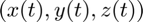 in phase space using plot3.
plot3(xa(:,1),xa(:,2),xa(:,3))
grid on
title('Solution curve')
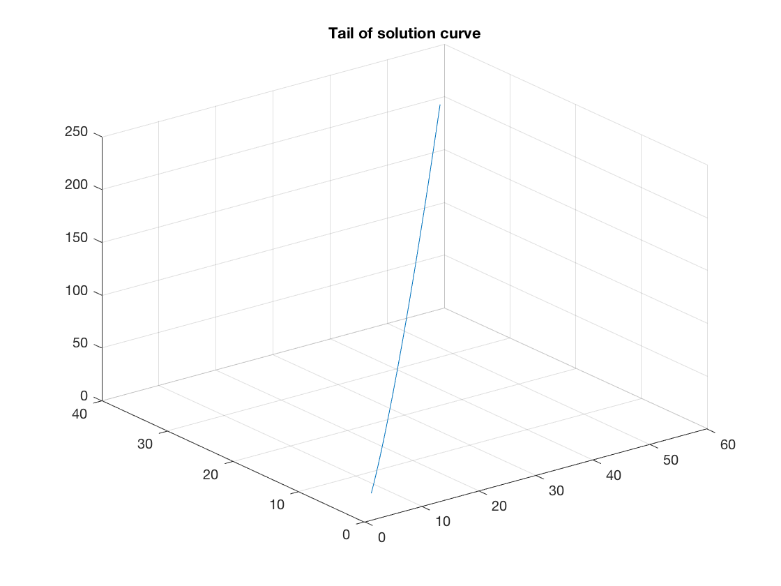
Plotting the tail
Suppose I just want to plot the part which corresponds approximately to the time interval ![$[1,1.5]$](plotting_part_of_solution_eq13765030470446389120.png) . Remember that the
. Remember that the  produced by ode45 is a vector with a lot of components. I want to know which component corresponds approximately to
  . One way is to look at the values of , but with a very long list of values this wouldn't be easy. So first I'll find how many components has, using the command size.
size(t)
ans =

    69     1
This tells me that has 69 rows and 1 column. Now I do some guessing: t(46) is two-thirds down the list of components of so I can look at it.
t(46)
ans =

    0.8747
I look at components with slightly larger index:
t(47:50)
ans =

    0.9122
    0.9497
    0.9872
    1.0247
I see that t(49) and t(50) are the closest, one a little larger, the other a little smaller than 1. I'll use 49 as my index. (You can probably do this more elegantly using the Events option.) So I can plot the tail of the solution curve with the following command.
plot3(xa(49:69,1),xa(49:69,2),xa(49:69,3))
grid on
title('Tail of solution curve')