Differential Equations with Maple Chapter 8
Contents
A case where ode45 does not give a good answer.
We look at the initial value problem

First we calculate the exact solution. This is a linear equation so it is easy to solve.
syms x
y = simplify(dsolve('Dy = y - 3*exp(-2*x), y(0) = 1', 'x'))
y =

1/exp(2*x)
Now we use ode45 to find a numeric solution.
f = @(x,y) y - 3*exp(-2*x);
[ta,ya] = ode45(f,[0,16],1);
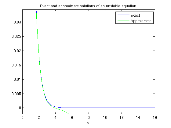
We plot the exact solution and approximate one together.
ezplot(y,[0,16]), hold on
plot(ta,ya,'g'),
title 'Exact and approximate solutions of an unstable equation'
legend({'Exact', 'Approximate'})
hold off

The solutions are the same until about x=3 then spread apart. The reason for this is that the problem is unstable. When you can't calculate the exact solution, you can calculate the numerical solution with greater accuracy, then compare. If the two results are not fairly close, the first one is probably not very accurate. We do this for this example, using odeset to improve the accuracy.
options = odeset('AbsTol', 1e-10, 'RelTol', 1e-10);
[tb,yb] = ode45(f,[0,16],1,options);
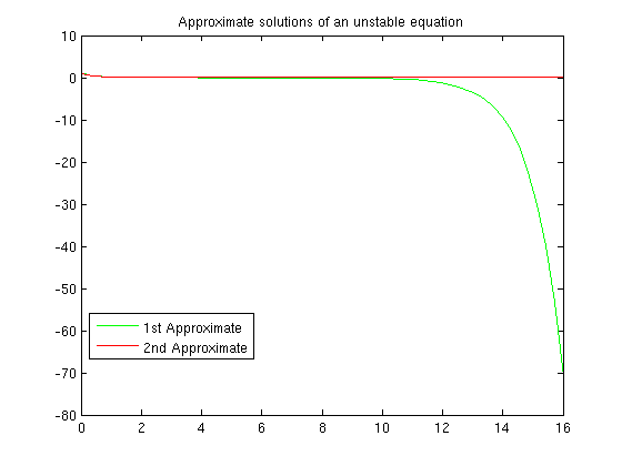
plot(ta,ya,'g'), hold on
plot(tb,yb,'r')
title 'Approximate solutions of an unstable equation'
legend({'1st Approximate','2nd Approximate'},'Position',[0.1572 0.2304 0.235 0.09836])
hold off

We see the two solutions start to differ between x=3 and x=4. At x=10 the difference starts to increase rapidly. From this, without knowing the exact solution, we could conclude that the first solution is probably not very accurate for x>10. By x=16 the difference is very large.
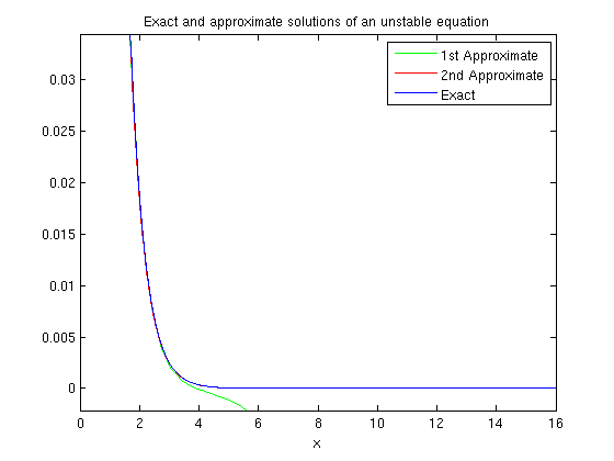
Here are the graphs of the two approximate solutions and the exact one. The more accurate approximate solution agrees with the exact one on this interval.
options = odeset('AbsTol', 1e-10, 'RelTol', 1e-10);
[tb,yb] = ode45(f,[0,16],1,options);
plot(ta,ya,'g'), hold on
plot(tb,yb,'r')
ezplot(y,[0,16])
title 'Exact and approximate solutions of an unstable equation'
legend({'1st Approximate','2nd Approximate','Exact'})
hold off
