Plotting the solution of the heat equation as a function of x and t
Contents
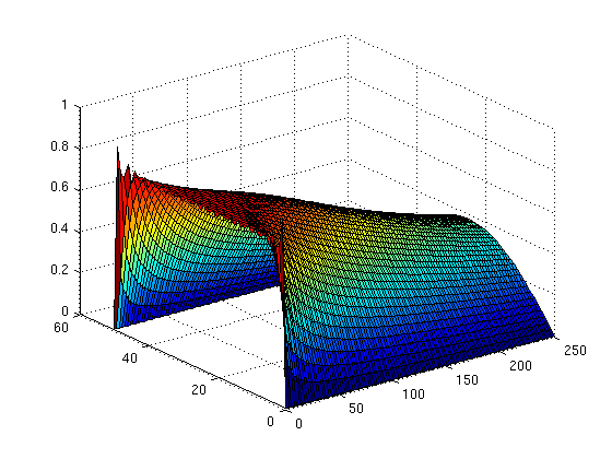
Here are two ways you can use MATLAB to produce the plot in Figure 10.5.5 of Boyce and DiPrima. In Example 1 of Section 10.5, the solution has been found to be be
For the plot, take  .
.
First method, defining the partial sums symbolically and using ezsurf
Unfortunately, I haven't figured out how to get ezsurf to do the graph in a reasonable amount of time using an anonymous function (the kind defined with @) but an inline function works.
syms x t n
u = inline((80/pi)*symsum(exp(-(2*n-1)^2*pi^2*t/2500)*sin((2*n-1)*pi*x/50)/(2*n-1),n,1,20));
ezsurf(u,[0 250 0 50])
title('')
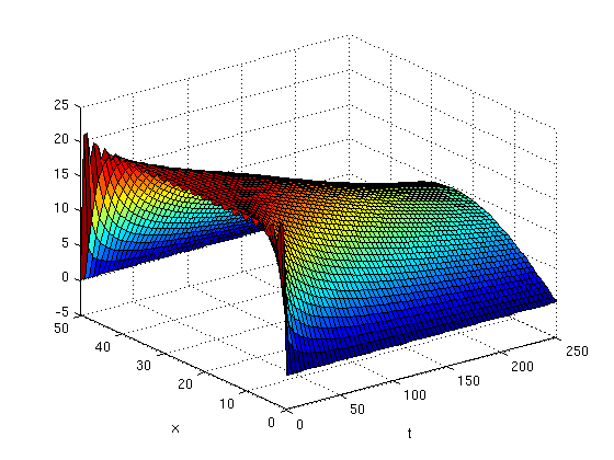
Second method, using surf
I start by defining the grid of x and t values where the values of u will be computed. Be careful not to use too many points in your meshgrid command; if you do you won't get a clear plot.
x = linspace(0,50,50); t = linspace(0,250,100); [X,T]= meshgrid(x,t);
Alternatively, I could create the meshgrid by giving the command
[X,T]= meshgrid(0:1:50,0:2.5:250);
Next I define u using a for loop to add terms, starting with u=0.
u=0;
for n=1:20
    u = u + exp(-(2.*n-1).^2.*pi.^2.*T./2500).*sin((2.*n-1).*pi.*X./50)./(2.*n-1);
end
surf(T,X,u)