Lab 03: Dice Rolling, Compound Interest
The goal of this lab assignment to allow you to explore repeated
execution by writing Python programs that utilize for and while
loops along with lists to simulate dice rolling and compound
interest.
For this assignment, record your work in a Jupyter Notebook and upload it to the form below by 11:59 PM Friday, February 14.
Activity 0: Starter Notebook
To help you get started, we have provided you with a starter notebook, which you can download and then use to record your answers. To utilize the starter notebook, download it to wherever you are running Jupyter Notebook and then use the Jupyter Notebook interface to open the downloaded file.
The starter notebook is already formatted for all the various sections you need to fill out. Just look for the red instructions that indicates were you need to write text or the cyan comments that indicate where you need to write code.
Activity 1: Dice Rolling Simulation
For the first activity, you are to simulate rolling a multiple-sided die multiple times to see its distribution of outcomes. To do so, we will use Python's random.randint function to generate a series of random integers and then store these dice rolls into a list for plotting:
Function
To simulate dice rolling, you will need to complete the following function:
import random

def simulate_dice(rolls, sides=6):
    ''' Simulate dice rolls '''
    results = []

    # TODO: Initialize results list to zeroes

    # TODO: Simulate dice rolls
    return results
This function takes the number of rolls to simulate and the number of
sides each die has.
Your first TODO is to initialize the results list to contain enough
zeroes for each possible side (ie. die roll). For instance, if sides is
6, we may wish to initialize the results to contain the following:
[0, 0, 0, 0, 0, 0, 0]
Note, we pad the results list by one item because we want to be able to
roll from 1 to the number of sides. The idea is that if we roll say a
2 we would increment results[2] by one to keep track of the number
times we rolled a 2.
results[2] += 1
Your next TODO is to simulate the dice rolls by using the
random.randint function to generate a random number between 1 and the
number of possible sides. You should then update the appropriate item in
the results list to keep track of the number of times we rolled that
side.
Finally, return the final set of results.
Example
Here is an exammple simulate_dice in action:
>>> simulate_dice(100)
[0, 15, 19, 15, 20, 16, 15]
Plotting
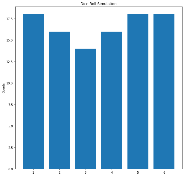
Once you have a working simulate_dice function, you can take the results
it produces and plot a bar graph (as shown above). To do so, you will
need to complete the following function:
import matplotlib.pyplot as plt

def plot_dice_rolls(results, sides):
    ''' Plot a bar graph of the dice roll simulation results '''
    plt.figure(figsize=(10, 10))

    # TODO: plot a bar where x coordinates are the sides and y
    # coordinates are the results of the simulation

    plt.ylabel('Counts')
    plt.title('Dice Roll Simulation')
The TODO you need to complete is to call the plot.bar graph with the
two following arguments:
-
x coordinates: This should be a range from
1to the number ofsides. For instance ifsidesis6, then you want a range that consists of:[1, 2, 3, 4, 5, 6] -
y coordinates: This should be the provided
resultsexcluding the initial0. For instance, if theresultswere[0, 15, 19, 15, 20, 16, 15]then you want to pass the following argument:[15, 19, 15, 20, 16, 15]
Once you have a working plot_dice_rolls function, you can do the
following to produce a bar graph:
sides   = 6
rolls   = 100
results = simulate_dice(rolls, sides)
plot_dice_rolls(results, sides)
Interaction
Your last task is to create a run_dice_simulation function that uses both
simulate_dice_rolls and plot_dice_rolls to simulate rolling dice
and then plotting them:
from ipywidgets import interact

def run_dice_simulation(rolls, sides):
    ''' Simulate dice rolls and then plot the results '''
Once you have a working run_dice_simulation function, you can use it to
create an interactive widget with the following code:
interact(run_dice_simulation, rolls=(1, 1000), sides=(2, 20))
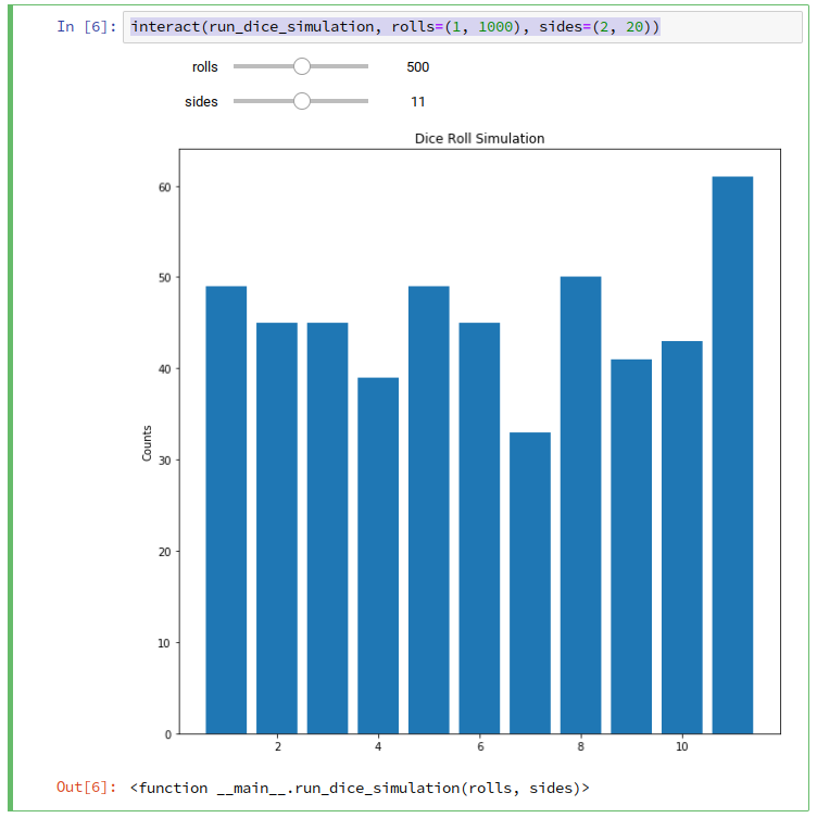
This will allow you to run your simulation with a different number of
rolls and with dice with different number of sides.
Reflection
After you have completed the program above, answer the following questions:
-
Describe the flow control of your program. What sort of conditional or repeated execution statements did you use?
-
Use your code to run a few simulations of rolling dice. If your application depended on unbiased or a fair distribution of results, would Python's default random number generator suffice? Explain.
Activity 2: Compound Interest Simulation
For the second activity, you are to simulate the calculation of compound interest so you can answer the question:
Given a starting principal and annual interest rate, how many years will it take for you to grow your principal to a target amount?
Once again, we will use functions, loops, and lists to produce a plot as shown below:
Function
To simulate the calculation of compound interest, you will need to complete the following function:
def simulate_compound_interest(principal, rate, target):
    ''' Simulate compound interest '''
    years    = 0
    interest = 0
    totals   = [principal]

    print('Years Principal Interest')
    print(f'{years:5} {principal:9.2f} {interest:8.2f}')

    # TODO: Compute compound interest until total principal exceeds target

    print(f'After {years} years you will have ${principal:.2f}')
    return totals
As can be seen, the initial bookkeeping variables are defined for you. The
years variable keeps track how many years have passed, while the
interest is used to store the amount of interest for the current year.
The totalslist is used to keep track of the principal for each year.
Likewise, we have provided you with some formatted strings so you can output a simple table as shown below.
Your TODO is to use a loop that updates the principal with the
amount of annual interest generated until the principal reaches or
surpasses the target using the following formula:
AnnualInterest = OldPrincipal * InterestRate
NewPrincipal   = OldPrincipal + AnnualInterest
After computing the updated principal, you should print out another entry
in the output table using the following code:
print(f'{years:5} {principal:9.2f} {interest:8.2f}')
Be sure to increment the years appropriately and append the principal
to the totals list.
Example
Here is an exammple simulate_compound_interest in action:
>>> simulate_compound_interest(1000, 0.05, 2000)
Years Principal Interest
    0   1000.00     0.00
    1   1050.00    50.00
    2   1102.50    52.50
    3   1157.62    55.12
    4   1215.51    57.88
    5   1276.28    60.78
    6   1340.10    63.81
    7   1407.10    67.00
    8   1477.46    70.36
    9   1551.33    73.87
   10   1628.89    77.57
   11   1710.34    81.44
   12   1795.86    85.52
   13   1885.65    89.79
   14   1979.93    94.28
   15   2078.93    99.00
After 15 years you will have $2078.93
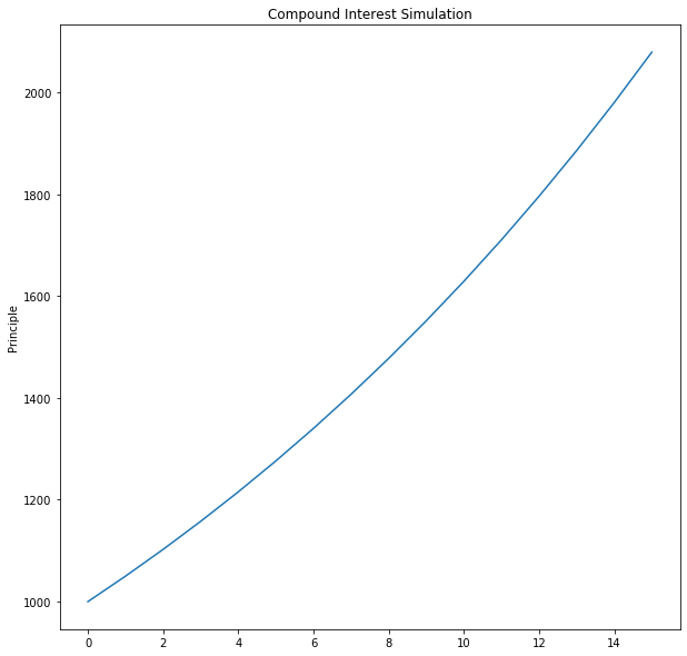
Plotting
Once you have a working simulate_compound_interest function, you can take
the totals it produces and plot a line graph (as shown above). To do
so, you will need to complete the following function:
import matplotlib.pyplot as plt

def plot_compound_interest(totals):
    ''' Plot a line graph of compound interest simulation totals '''
    plt.figure(figsize=(10, 10))

    # TODO: plot line graph where x coordinates are the years and y
    # coordinates are the yearly totals from the simulation

    plt.plot(range(len(totals)), totals)
    plt.ylabel('Principal')
    plt.title('Compound Interest Simulation')
The TODO you need to complete is to call the plot.plot graph with the
two following arguments:
-
x coordinates: This should be a range from
1to the number of items in thetotalslist. For instance iftotalshad4items, you would a range that consists of:[0, 1, 2, 3] -
y coordinates: This should be the provided
totals.
Once you have a working plot_compound_interest function, you can do the
following to produce a line graph:
principal = 1000
rate      = 0.05
target    = 2000

totals    = simulate_compound_interest(principal, rate, target)
plot_compound_interest(totals)
Note, this will output both the table and the plot.
Interaction
Your last task is to create a run_cpi_simulation function that uses both
simulate_compound_interest and plot_compound_interest to simulate calculating
compound interest and then plotting the yearly totals:
from ipywidgets import interact

def run_cpi_simulation(principal, rate, target):
    ''' Simulate compound interest and plot totals '''
Once you have a working run_cpi_simulation function, you can use it to
create an interactive widget with the following code:
interact(run_cpi_simulation, principal='', rate=(0.0, 1.0, 0.05), target='')
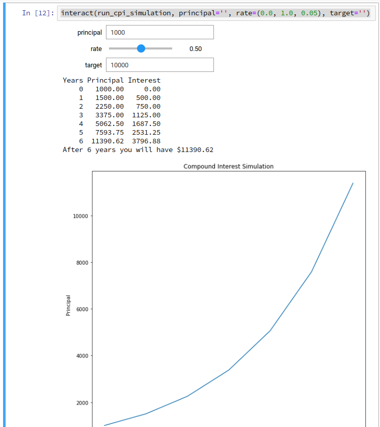
This will allow you to run your simulation with a different starting
principal, annual interest rate, and final target.
Reflection
After you have completed the program above, answer the following questions:
-
Describe the flow control of your program. What sort of conditional or repeated execution statements did you use?
-
Use your code to run a few simulations of compound interest. What is it important to invest early and for long periods of time?
Submission
Once you have completed your lab, submit your Jupyter Notebook using the form: