This is a real-world example in which parallelization will give a speed boost. Along the way, we'll show how to handle a situation in which an error occurs in one hard-to-find iteration of loop. We'll also discuss profiling R code for speed.
Here, we will compute finite gaussian mixture models for many thousands of continuous variables. The variables measure gene expression levels in breast cancer patients. This is useful in computing disease subtypes and diagnostic models.
This is just a rough description suitable for our purposes. For a formal treatment see, e.g.,
C. Fraley and A. Raftery, Model-based clustering, discriminant analysis, and density estimation, JASA, (2002) vol 97 (458) pp. 611 - 631.
Consider the following vector.
setwd("/Users/steve/Documents/Computing with Data/22_parallel/")
load("./Data/y.RData")
summary(y)
##    Min. 1st Qu.  Median    Mean 3rd Qu.    Max.
##    0.31    4.51    7.53    6.62    8.81   12.80
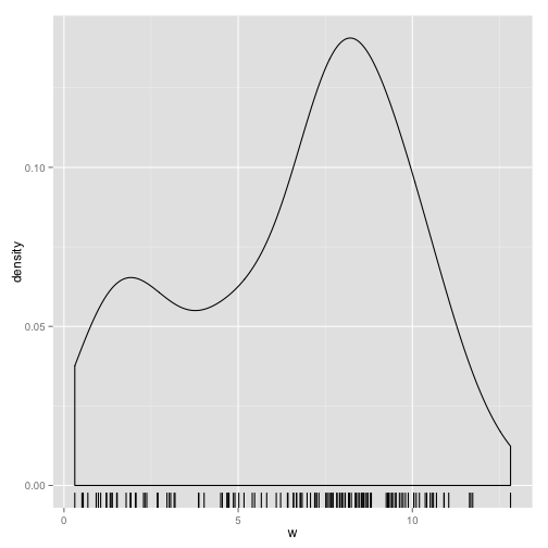
Plot the density distribution of y.
library(ggplot2)
ggplot(data = data.frame(w = y), aes(x = w)) + geom_density() + geom_rug()
It looks like a pair of normal distributions with different means. The mixture model methodology is designed to identify the different distributions that combine to make up the distribution of the sample. This can be thought of as a form of clustering. Here, we'll only consider mixture models in which the components are gaussian distributions with varying means and standard deviations.
Given a vector x, the mixture model methodology applied to x will attempt to find the set of gaussian components (one or more components) that best fit the distribution of x. This employs the Expectation-Maximization (EM) algorithm to maximize likelihood. This is a type of one-dimensional clustering. The best fit may be with 1 component, 2 components, etc.
Consider another example.
load("./Data/v.RData")
ggplot(data = data.frame(w = v), aes(x = w)) + geom_density() + geom_rug()
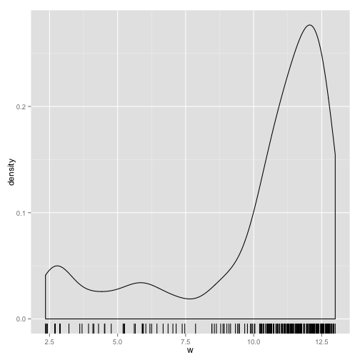
Clearly there is one component with a mean around 12. We could have one component with mean around 6 and large standard deviation, or 2 other components with means around 7 and 2.7. One of those models is likely to fit the data the best.
To execute gaussian mixture model fits we'll use the library mclust.
library(mclust)
## Package 'mclust' version 4.2
Run a fit on the two vectors we've inspected.
mc_y <- Mclust(y)
summary(mc_y, parameters = T)
## ----------------------------------------------------
## Gaussian finite mixture model fitted by EM algorithm
## ----------------------------------------------------
##
## Mclust E (univariate, equal variance) model with 2 components:
##
##  log.likelihood   n df    BIC    ICL
##          -316.6 130  4 -652.7 -665.3
##
## Clustering table:
##  1  2
## 41 89
##
## Mixing probabilities:
##      1      2
## 0.3121 0.6879
##
## Means:
##     1     2
## 2.645 8.417
##
## Variances:
##    1    2
## 2.69 2.69
Mclust will find the maximum likelihood and try to minimize the complexity of the model (number of degrees of freedom).
Now consider the second vector.
mc_v <- Mclust(v)
summary(mc_v, parameters = T)
## ----------------------------------------------------
## Gaussian finite mixture model fitted by EM algorithm
## ----------------------------------------------------
##
## Mclust V (univariate, unequal variance) model with 3 components:
##
##  log.likelihood   n df   BIC   ICL
##          -491.4 251  8 -1027 -1085
##
## Clustering table:
##   1   2   3
##  59 116  76
##
## Mixing probabilities:
##      1      2      3
## 0.2434 0.4992 0.2574
##
## Means:
##      1      2      3
##  5.429 11.202 12.485
##
## Variances:
##       1       2       3
## 5.98563 0.62831 0.06515
The best split here was with 3 components.
Load the matrix of expression values.
load("./Data/expression_matrix.RData")
dim(expression_matrix)
## [1] 22283 1269
expression_matrix[1:3, 1:4]
##           GSM79114 GSM79118 GSM79119 GSM79120
## 1007_s_at    9.990    9.536   10.189    9.682
## 1053_at      4.241    5.957    5.579    5.334
## 117_at       3.406    3.615    3.573    3.741
Rows correspond to the genes.
We'll want to do Mclust on 100 rows. We may need to parallelize it so set it up with foreach rather than lapply or a plyr method.
Load the necessary libraries.
library(foreach)
library(iterators)
Set up the matrix of the first 50 rows as an iterator.
mat_test <- iter(expression_matrix[1:100, ], by = "row")
Run foreach over the rows and execute Mclust. Time this execution.
system.time(mclust_test <- foreach(r = mat_test) %do% Mclust(r))
There is a problem here in that for some genes, Mclust may not work. In fact, running it may give an error when the algorithm can't be applied.
By default, when running a series of R commands, when an error is encountered, an error message is printed and a stop command is given, prohibiting further exection. error catching is a general term for methods to keep track of errors when they occur, but not cause a stop. The basic function that R has for doing this is try.
name_it <- function(x, y) {
    names(x) <- y
    x
}
w <- name_it(c(1, 2), c("a", "b", "c"))
w
# error occurs
Enclose the command or function with try
name_it <- function(x, y) {
    names(x) <- y
    x
}
z <- try(name_it(c(1, 2), c("a", "b", "c")))
z
## [1] "Error in names(x) <- y : \n  'names' attribute [3] must be the same length as the vector [2]\n"
## attr(,"class")
## [1] "try-error"
## attr(,"condition")
## <simpleError in names(x) <- y: 'names' attribute [3] must be the same length as the vector [2]>
Here, an error message was given but z was assigned a value. Inside a block of other commands, like a function, processing commands would continue.
In a large collection of assignments, how do we recognize the ones that result from errors?
class(z)
## [1] "try-error"
This has a special class.
try is a function that if given any valid input will simply return that same input. If given an "error" as input, it returns a special object of class "try-error".
mat_test <- iter(expression_matrix[1:100, ], by = "row")
system.time(mclust_test <- foreach(r = mat_test) %do% try(Mclust(r)))
## Warning: no assignment to 2,3,5
## Warning: there are missing groups
## Warning: there are missing groups
## Warning: there are missing groups
## Warning: there are missing groups
## Warning: there are missing groups
## Warning: there are missing groups
## Warning: there are missing groups
## Warning: there are missing groups
## Warning: there are missing groups
## Warning: no assignment to 1,2,4
## Warning: no assignment to 2,3,4,5
## Warning: best model occurs at the min or max # of components considered
## Warning: no assignment to 2,3,4
## Warning: no assignment to 3,4,6
## Warning: no assignment to 2,3,4
## Warning: no assignment to 1,3,4,5
## Warning: no assignment to 1,3,4,5
## Warning: best model occurs at the min or max # of components considered
## Warning: best model occurs at the min or max # of components considered
## Warning: optimal number of clusters occurs at min choice
## Warning: best model occurs at the min or max # of components considered
## Warning: optimal number of clusters occurs at min choice
## Warning: best model occurs at the min or max # of components considered
## Warning: optimal number of clusters occurs at min choice
## Warning: best model occurs at the min or max # of components considered
## Warning: optimal number of clusters occurs at min choice
## Warning: best model occurs at the min or max # of components considered
## Warning: optimal number of clusters occurs at min choice
##    user  system elapsed
## 123.994   2.842 126.840
This hit an error but kept running, completing in around 2 minutes.
Now separate the failures from the successes. We do this by finding the return values that have class "try-error".
Remember that foreach by default returns a list.
table(sapply(mclust_test, class))
##
##    Mclust try-error
##        99         1
One error.
bad <- which(sapply(mclust_test, class) == "try-error")
good_mclust_test <- mclust_test[-bad]
First load doMC and register the parallel workers.
library(doMC)
## Loading required package: parallel
registerDoMC()
Parallelize the foreach
mat_test <- iter(expression_matrix[1:100, ], by = "row")
system.time(mclust_test_par <- foreach(r = mat_test) %dopar% try(Mclust(r)))
##    user  system elapsed
##  37.499   0.439  97.906
We got a good speedup.
Note that although the inputs may have been scrambled and sent to different processors, the output list will have objects lined up with the corresponding input.
A few additional steps are needed to set up a multi-node cluster and run foreach in this cluster environment. A standard package for parallelization is snow, which is installed at CRC.
After loading the package with library(snow) you need to initialize a cluster to use. There are different functions depending on the method by which the nodes (individual computers) are linked together. In CRC they use MPI, so the cluster object is created by
cl <- makeMPIcluster(count)
where count refers to the number of nodes you want to use.
The snow package has some functions for parallel apply, split and some other operations. It may be easiest, though, to do the extra steps needed to run an instance of foreach.
foreachThere is another package that handels this, namely doSNOW. After installing the package, run
library(doSNOW)
registerDoSNOW(cl)
foreachNow simply run your foreach application with %dopar% and it will use the cluster to evaluate it. Note that if the function after the %dopar% makes use of a package beyond base R you will need to tell the cluster to load the library on each of the worker nodes. This is done with the option .packages = ... inside of the foreach call.
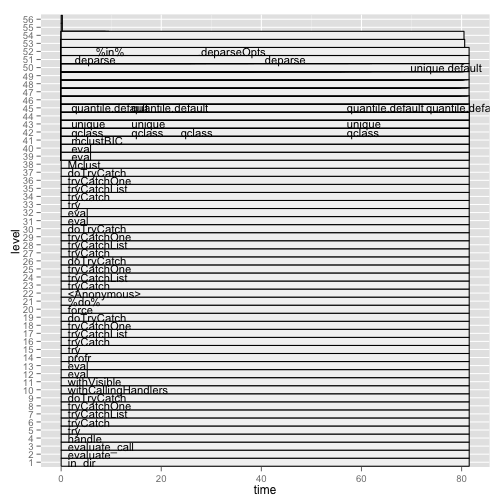
Profiling code is a method of assessing the processing time each step of a process takes. R's method of profiling is not easy to interpret. I'll illustrate a package profr that works a little better.
library(profr)
x <- foreach(i = 1:1000, .combine = "cbind") %do% rnorm(3)
prof1_out <- profr(x <- foreach(i = 1:1000, .combine = "cbind") %do% rnorm(3))
ggplot(prof1_out)
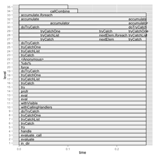
mat_test <- iter(expression_matrix[1:10, ], by = "row")
prof2_out <- profr(mclust_test_par <- foreach(r = mat_test) %do% try(Mclust(r)))
## Warning: no assignment to 2,3,5
## Warning: there are missing groups
## Warning: there are missing groups
## Warning: there are missing groups
## Warning: there are missing groups
## Warning: there are missing groups
## Warning: there are missing groups
## Warning: there are missing groups
## Warning: there are missing groups
## Warning: there are missing groups
## Warning: no assignment to 1,2,4
## Warning: no assignment to 2,3,4,5
## Warning: best model occurs at the min or max # of components considered
## Warning: no assignment to 2,3,4
head(prof2_out)
##                f level  time start   end  leaf source
## 8         in_dir     1 81.52     0 81.52 FALSE   <NA>
## 9       evaluate     2 81.52     0 81.52 FALSE   <NA>
## 10 evaluate_call     3 81.52     0 81.52 FALSE   <NA>
## 11        handle     4 81.52     0 81.52 FALSE   <NA>
## 12           try     5 81.52     0 81.52 FALSE   base
## 13      tryCatch     6 81.52     0 81.52 FALSE   base
ggplot(prof2_out)