In many problems the possible variables that may effect an outcome are extensive. Being able to screen these effiociently, perhaps even in parallel is very important. This involves setting up the data in a particular way. First, a discussion of varying ways to represent data.
In many settings a data collection amounts to recording measurements of a particular variable. If we're recording several years of expenditures per state and in various categories of expenses then a single data element will have characteristics: (state, year, category, amount). There are multiple ways to organize this into a tabular array (data frame). We could have years as the columns and rows determined by pairs of (state, category), etc. Probably the most flexible format has one column for each of the attributes listed above. This gives lots of records and few columns, but by having a variable for each possible attribute we can study variables in a wide variety of ways.
Goal: Identify the genes whose expression values significantly vary over tumor grade in the Metabric breast cancer data.
Earlier, we inspected the patient clinical characteristics from the Metabric data, using it to illustrate the transformations we need to do to real data. For this problem we also need gene expression data from the patients' tumors.
setwd("~/Documents/Computing with Data/9_Lists_of_data_frames/")
clin_data1_df <- read.csv("./Data/metabric_published_clinical.csv", stringsAsFactors = F)
str(clin_data1_df)
## 'data.frame':    1992 obs. of  8 variables:
##  $ X                         : int  1 2 3 4 5 6 7 8 9 10 ...
##  $ sample                    : chr  "MB.0002" "MB.0008" "MB.0010" "MB.0035" ...
##  $ age_at_diagnosis          : num  43.2 77 78.8 84.2 85.5 ...
##  $ last_follow_up_status     : chr  "a" "d-d.s." "d-d.s." "d" ...
##  $ menopausal_status_inferred: chr  "pre" "post" "post" "post" ...
##  $ grade                     : chr  "3" "3" "3" "2" ...
##  $ size                      : chr  "10" "40" "31" "28" ...
##  $ stage                     : chr  "1" "2" "4" "2" ...
load("./Data/expr_matrix_Metabric.RData")
expr_matrix_Metabric[1:5, 1:4]
##              MB.0362 MB.0346 MB.0386 MB.0574
## ILMN_1802380   8.677   9.654   9.034   8.815
## ILMN_1893287   5.299   5.379   5.606   5.316
## ILMN_1736104   5.431   5.199   5.449   5.309
## ILMN_1792389   6.075   6.688   5.911   5.629
## ILMN_1854015   5.596   6.010   5.684   5.480
The expression matrix has patients listed in the columns and genes in the rows. the cells are measurements of the expression level of that gene in the patient's tumor. Gene expression is measured on a continous scale. (More properly, the codes like ILMN_1802380 represent features on a microarray that bind to the mRNA produced by the gene.) There are 48787 features in this array and we want to know which ones are effected by tumor grade.
What is the form of the statistical test we want to use? Tumor grade is categorical and gene expression is continuous. We test genes for variation across grades by a linear regression with expression as the response variable and grade as the covariate:
lm(expression ~ grade, data = ?)
How we set up the problem is key. "expression" must be a variable name for the expression level of a particular gene. We could transpose the matrix and make it a data.frame producing a named variable for each gene. But how do we insert all of these different names into linear equations?
The cells in the expression matrix are determined by (sample, feature, value). If we had the data in long form (and included grade) in an object df_long, we could test dependence of a feature x using the formula
lm(value ~ grade, data = df_long restricted to feature = x)
Varying the features, the variable in the formula is the same and the data changes. This is the easiest way do this large batch operation.
In fact it will be easiest to set this up as a list of dataframes, one component for each feature. Generating the full object df_long is unnecessary and would take a lot of processing time.
We will need to include grade in the analysis, so let's check it's format and extract it from the clinical data.
table(clin_data1_df$grade)
##
##    1    2    3 null
##  170  775  957   90
clin_data1_df[clin_data1_df$grade == "null", "grade"] <- NA
table(clin_data1_df$grade)
##
##   1   2   3
## 170 775 957
sum(is.na(clin_data1_df$grade))
## [1] 90
clin_data1_df$grade <- factor(clin_data1_df$grade)
grade_df <- subset(clin_data1_df, select = c(sample, grade))
We know from experience that many of the genes in the data will have very little change in expression across the samples, so aren't very interesting for this purpose. We'll filter these out.
iqr_vals <- apply(expr_matrix_Metabric, 1, IQR)
summary(iqr_vals)
##    Min. 1st Qu.  Median    Mean 3rd Qu.    Max.
##   0.012   0.171   0.203   0.348   0.450   5.690
# restrict to the features with IQR at least 0.5
expr_filt_matrix <- expr_matrix_Metabric[iqr_vals > 0.5, ]
Now, the rows of this matrix are the features we will test for dependence on grade.
feature_filt <- rownames(expr_filt_matrix)
For each such feature we want a data.frame containing the information (sample, grade, expr value). We'll put the data.frames in a list indexed over the features. We have grade in a separate data.frame, so it's easiest to include it by merging.
all_samples <- colnames(expr_filt_matrix)
system.time(expr_df_L <- lapply(feature_filt, function(x) {
    df1 <- data.frame(sample = all_samples, value = expr_filt_matrix[x, ])
    df2 <- merge(df1, grade_df)
    df2
}))
# Takes 307 seconds to run
names(expr_df_L) <- feature_filt
save(expr_df_L, file = "expr_df_L.RData")
load("expr_df_L.RData")
Look at one component.
head(expr_df_L[[1]])
##    sample value grade
## 1 MB.0000 9.738     3
## 2 MB.0002 9.014     3
## 3 MB.0005 7.963     2
## 4 MB.0006 8.177     2
## 5 MB.0008 8.050     3
## 6 MB.0010 8.386     3
names(expr_df_L)[1]
## [1] "ILMN_1802380"
head(expr_df_L[[2]])
##    sample value grade
## 1 MB.0000 6.470     3
## 2 MB.0002 5.749     3
## 3 MB.0005 5.553     2
## 4 MB.0006 5.391     2
## 5 MB.0008 5.531     3
## 6 MB.0010 5.453     3
names(expr_df_L)[2]
## [1] "ILMN_1792389"
We have a list of dataframes and want to run a linear model for value ~ grade in each.
system.time(grad_gene_lm_L <- lapply(expr_df_L, function(df) {
    lm1 <- lm(value ~ grade, data = df)
    lm1
}))
##    user  system elapsed
##  35.688   1.184  36.873
names(grad_gene_lm_L) <- names(expr_df_L)
What we have from the list now is a big collection of linear model fits.
class(grad_gene_lm_L[[100]])
## [1] "lm"
names(grad_gene_lm_L[[100]])
##  [1] "coefficients"  "residuals"     "effects"       "rank"
##  [5] "fitted.values" "assign"        "qr"            "df.residual"
##  [9] "na.action"     "contrasts"     "xlevels"       "call"
## [13] "terms"         "model"
summary(grad_gene_lm_L[[100]])
##
## Call:
## lm(formula = value ~ grade, data = df)
##
## Residuals:
##     Min      1Q  Median      3Q     Max
## -1.5098 -0.2654 -0.0144  0.2723  2.0113
##
## Coefficients:
##             Estimate Std. Error t value Pr(>|t|)
## (Intercept)   7.0804     0.0327  216.74  < 2e-16 ***
## grade2       -0.1073     0.0361   -2.97    0.003 **
## grade3       -0.2286     0.0355   -6.45  1.4e-10 ***
## ---
## Signif. codes:  0 '***' 0.001 '**' 0.01 '*' 0.05 '.' 0.1 ' ' 1
##
## Residual standard error: 0.426 on 1899 degrees of freedom
##   (90 observations deleted due to missingness)
## Multiple R-squared: 0.031,   Adjusted R-squared: 0.0299
## F-statistic: 30.3 on 2 and 1899 DF,  p-value: 1.06e-13
names(summary(grad_gene_lm_L[[100]]))
##  [1] "call"          "terms"         "residuals"     "coefficients"
##  [5] "aliased"       "sigma"         "df"            "r.squared"
##  [9] "adj.r.squared" "fstatistic"    "cov.unscaled"  "na.action"
We want to identify genes that are most significant. Most convenient is to use the F statistic, since all of these have the same degrees of freedom. How do we pull out the F statistic?
summary(grad_gene_lm_L[[100]])$fstatistic
##   value   numdf   dendf
##   30.35    2.00 1899.00
summary(grad_gene_lm_L[[100]])$fstatistic[1]
## value
## 30.35
Go back to the full list of lm objects, and use a sapply application to extract the F statistics.
gene_fstats <- sapply(grad_gene_lm_L, function(x) summary(x)$fstatistic[1])
names(gene_fstats) <- names(grad_gene_lm_L)
summary(gene_fstats)
##    Min. 1st Qu.  Median    Mean 3rd Qu.    Max.
##     0.0     4.1    14.7    30.3    40.7   357.0
Order these by F statistic.
gene_fstats_srt <- sort(gene_fstats, decreasing = T)
gene_fstats_srt[1:20]
## ILMN_1683450 ILMN_1673721 ILMN_1801939 ILMN_1680955 ILMN_1801257
##        356.8        325.4        321.4        320.7        318.6
## ILMN_2413898 ILMN_2357438 ILMN_2301083 ILMN_1670238 ILMN_1747016
##        318.6        317.5        316.2        315.7        313.6
## ILMN_1685916 ILMN_2212909 ILMN_1796589 ILMN_1663390 ILMN_1786125
##        313.1        310.1        306.8        305.5        304.8
## ILMN_1684217 ILMN_1714730 ILMN_2202948 ILMN_2042771 ILMN_1751444
##        304.0        303.1        301.1        295.0        294.6
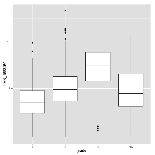
For the most significant one, let's do a boxplot.
library(ggplot2)
box_top_gene_plot <- ggplot(data = expr_df_L[["ILMN_1683450"]], aes(x = grade,
    y = value)) + geom_boxplot() + ylab("ILMN_1683450")
box_top_gene_plot
What we've seen is an example of taking a large problem, coded in a big collection of data, splitting the data into smaller pieces by a uniform routine, applying a function to each piece, and then assembling the results into a usable form, like a vector or single data.frame.
Setting up the problem this way will enable you to parallelize such a problem rather easily. There are parallel versions of lapply that let you use multiple cores to analyze all of the cases.
This is also in line with the Big Data map reduce methodology used to analyze distributed data. Statistics with distributed data is much more delicate, but learning this split-apply paradigm will teach you to think the right way about these problems.