Goal: This case introduces trend behavior in a time series and some techniques for eliminating such a trend. Since some forecasting models require any trend be removed from the data, data detrending is an important aspect of business forecasting. Specifically, this case introduces how to:

• Generate naive forecasts using Excel
• Examine Trend in a Time Series
• Remove a Linear Trend by Data Differencing.

The spreadsheet for this problem is CH1_Case2.xls. It contains the following data:

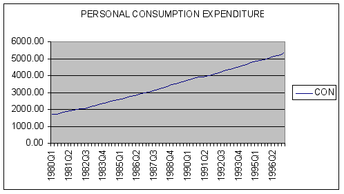
The series CON is quarterly personal consumption expenditure data from quarter 1 of 1980 through quarter 1 of 1997.

.

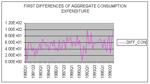
The series DIFF_CON is the first-difference of the CON series, which is designed to eliminate any linear trend in the original series. Using a spreadsheet we calculated first differences as follows:

The series FORECAST_CON_ONE contains forecasts of CON using the first-naïve forecasting model of Chapter One, and is calculated using a spreadsheet as:

The series FORECAST_CON_TWO contains forecasts of CON using the second-naïve forecasting model of Chapter One, and is calculated using a spreadsheet as:

Note how the second "naive" forecasting model adds an adaptive structure to the first naïve model. In addition, we have assumed the adjustment parameter P is 0.5 for the second naive model.

The series FORECAST_DIFFCON_ONE contains forecasts of DIFF_CON using the first-naïve forecasting model of Chapter One, and is calculated using a spreadsheet as:

The series FORECAST_CON_TWO contains forecasts of DIFF_CON using the second-naïve forecasting model of Chapter One, and is calculated using a spreadsheet as:

Examination of Trend in a Time Series

Trend in a time series is defined as the long-term change in the level of the data. Some forecasting models are designed to model trend behavior in a time series, whereas other methods require the data to be stationary, i.e., display no appreciable trend. Accordingly, in some cases, researchers are required to remove or detrend a given time series. A common practice to remove any linear trend is to first-difference the data, i.e., subtract successive observations of the levels of the data. This can easily be done in your favorite spreadsheet.

We next seek to plot our data. A time-series plot of the level and first-differences of aggregate consumption are shown below.

Question #1: Based upon examination of the time-series plot of CON and DIFF_CON, does first differencing of the data remove the trend present in the original series?

ANSWER:

We now want to examine some simple naïve forecasting methods and how they perform on data with and without trend. The first-naïve model simply assumes that the forecast for today is what was actually observed last period, and is incapable of tracking a linear trend. The second-naïve model adds to the first an adaptive structure that tracks the directions of change between last period and the period before, and is capable of tracking a linear trend in the data. Accordingly, we expect the second-naïve model to outperform the first when applied to data with a trend, since the first model ignores any trend behavior.

If our assertions about modeling trend are correct, we expect the first-naïve model to have a lower root-mean-squared-error (RMSE) for the linearly detrended series (DIFF_CON) and higher RMSE for the series with trend (CON).

Using Excel we calculated the RMSE for each forecasting outcome and is reported in the following table.

Question #2: Based upon examination of in-sample RMSE over the period 1980Q1-1997Q1, which forecasting method is more accurate and when?

ANSWER:

Question #3: Does your answer to Question 3 verify the assertion that the first-naïve model is best applied to data with no trend, and the second-naïve model is best applied to data with a trend?

ANSWER:

Question #1: How robust are the above results to the choice of the parameter P in the second naive model? Compare RMSEs for various choices of P where 0 < P < 1.

Question #2: Contrast and compare first- and second-differences of the CON data for the presence (absence) of any non-linear trend. Compare time-series plots of the two series and note how they compare with regard to being stationary.

Question #3: How can we forecast the level of a variable when our model requires the data to be first-differenced to produce stationarity? Explain.