Notebook 07: File I/O

Overview

The goal of this assignment is to allow you to practice reading data from files, performing some analysis on the data, and then presenting the data visually via plots and graphs in the Python programming language. Additionally, you will continue to practice decomposing large problems into smaller sub-problems in each of these activities.

To record your solutions and answers, create a new Jupyter Notebook titled Notebook07.ipynb and use this notebook to complete the following activities and answer the corresponding questions.

Make sure you label your activities appropriately. That is for Activity 1, have a header cell that is titled Activity 1. Likewise, use the Markdown cells to answer the questions (include the questions above the answer).

This Notebook assignment is due Midnight Friday, November 6, 2015 and is to be done individually.

Activity 0: Baby Names Dataset

For all the activities for this Notebook, you will be working on data from the Social Security Administration. In particular, you will be examining the most popular (top 1000) baby names from 1880 to 2014. Before you can analyze and visualize this data, however, you must first download the data from the Social Security Administration website, and then extract the information on your local computer.

To do this, you are to write the following functions:

ls(path=os.curdir, sort=True):

Given a path to a directory, this function prints the names of all the files in that directory. If sort is True, then the contents are printed in lexigraphical order.
head(path, n=10):

Given a path to a file, this function prints the first n lines in the file.
tail(path, n=10):

Given a path to a file, this function prints the last n lines in the file.
download_and_extract_zipfile(url, destdir):

Given a url (i.e. a uniform resource locator) to a zipfile, this function retrieves the file via a HTTP request and then extracts all the contents of the file to the specified destdir.

Code Skeleton

The following is a skeleton of the code you must implement to complete this activity.

# Imports

import os
import requests
import zipfile
import StringIO

# Constants

NATIONAL_DATA_URL = 'https://www.ssa.gov/oact/babynames/names.zip'
NATIONAL_DATA_DIR = 'national_baby_names'

STATE_DATA_URL    = 'https://www.ssa.gov/oact/babynames/state/namesbystate.zip'
STATE_DATA_DIR    = 'state_baby_names'

# Functions

def ls(path=os.curdir, sort=True):
    ''' Lists the contents of directory specified by path '''
    # TODO: Implement function

def head(path, n=10):
    ''' Lists the first n lines of file specified by path '''
    # TODO: Implement function

def tail(path, n=10):
    ''' Lists the last n lines of file specified by path '''
    # TODO: Implement function

def download_and_extract_zipfile(url, destdir):
    ''' Downloads zip file from url and extracts the contents to destdir '''
    # TODO: Request URL and open response content as ZipFile

    # TODO: Extract all zip data to destdir

Once you have implemented the download_and_extract_zipfile function, use it retrieve and extract both the national dataset and the state dataset to your local computer:

>>> download_and_extract_zipfile(STATE_DATA_URL, STATE_DATA_DIR)

Once you have implemented the ls, head, and tail functions, use them to explore the extracted datasets:

>>> ls(STATE_DATA_DIR)
AK.TXT
... SNIP ...
WY.TXT

>>> head('state_baby_names/IN.TXT')
IN,F,1910,Mary,619
IN,F,1910,Helen,324
IN,F,1910,Ruth,238
IN,F,1910,Dorothy,215
IN,F,1910,Mildred,200
IN,F,1910,Margaret,196
IN,F,1910,Thelma,137
IN,F,1910,Edna,113
IN,F,1910,Martha,112
IN,F,1910,Hazel,108

>>> tail('state_baby_names/IN.TXT')
IN,M,2014,Tryston,5
IN,M,2014,Tyreese,5
IN,M,2014,Tyrone,5
IN,M,2014,Vernon,5
IN,M,2014,Viktor,5
IN,M,2014,Waylen,5
IN,M,2014,Xavi,5
IN,M,2014,Yael,5
IN,M,2014,Zain,5
IN,M,2014,Zakary,5

Hints

The following are hints and suggestions that will help you complete this activity:

To get the contents of a directory or folder, you can use the os.listdir function.
When iterating over a file handle, each line contains the trailing newline, so use the str.strip method to remove any unnecessary whitespace.
To retrieve a file over HTTP, use the requests.get method on a URL. The contents of the response object can be accessed via: response.content.
To convert a string into a file object, use the StringIO.StringIO function.
To open a file object as a zipfile, use the zipfile.ZipFile function. To extract all the contents of the file, use the ZipFile.extractall method.

Questions

After completing the activity above, answer the following questions:

Retrieve the national dataset and extract it to NATIONAL_DATA_DIR. Explore the contents of the NATIONAL_DATA_DIR folder. How is the national dataset organized? What is the format of each individual file?
Retrieve the state dataset and extract it to STATE_DATA_DIR. Explore the contents of the STATE_DATA_DIR folder. How is the state dataset organized? What is the format of each individual file?

Activity 1: National Baby Names

For this activity, you are to process all of the files in the national dataset and generate two plots of your name from 1880 to 2014:

The first graph you should produce is a plot of the raw number of occurrences for each year.
The second graph you should produce is a plot of the percentage of occurrences for each year (how many times your name appeared relative to the total number of names).

Imports

To have the plots display inline inside the Jupyter Notebook, you must first execute the following command:

%matplotlib inline

Once this is done, any plots you generate will show us as an image inside the Notebook.

To access the plotting functions, you must perform the following import:

import matplotlib.pyplot as plt

Functions

To complete this activity, we can break the activity down into the following functions:

Count the occurrences in a year file
```
def count_occurrences_in_year(path, baby_name):
    ''' Return the number of occurrences for the baby_name and the total number of babies for the year file specified by path '''
```
Given the path to a year file and a target baby_name, return the number of occurrences for the baby_name and the total number of names for that year.

Once you have completed this function, you should be able to do the following:
```
>>> count_occurrences_in_year(os.path.join(NATIONAL_DATA_DIR, 'yob1880.txt'), 'Peter')
(496, 201484)
```
This means that the name Peter was given to 496 out of 201484 babies in the year 1880.
Count the occurrences in a range of years
```
def count_occurrences_in_years(path, baby_name, years):
    ''' Return a list of occurrences for the range of years in the data directory specified by path '''
```
Given the path to a directory containing the years data, list of years, and a target baby_name, return a list of all the occurrences of baby_name and the total number of names for each year. Internally, this function uses the count_occurrences_in_year function.

Once you have completed this function, you should be able to do the following:
```
>>> count_occurrences_in_years(NATIONAL_DATA_DIR, range(1880, 2015), 'Peter')
[(496, 201484),
 (428, 192700),
 (461, 221537),
 ... SNIP ...
 (1859, 3638838),
 (1833, 3608097),
 (1899, 3670151)]
```
This returns a list of pairs containing the number of occurrences of the name Peter along with the total number of names for each year from 1880 through 2014.
Plot the national occurrences
```
def plot_national_occurrences(data, years):
    ''' Plot the number of occurrences in the given range of years '''
```
Given the data returned from count_occurrences_in_years and a range of years, plot the number of occurrences for each year.

Once you have completed this function, you should be able to do the following:
```
>>> years = range(1880, 2015)
>>> data  = count_occurrences_in_years(NATIONAL_DATA_DIR, years, 'Peter')
>>> plot_national_occurrences(data, years)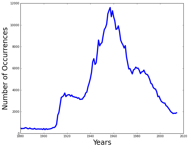
```
This shows the number of occurrences for the name Peter for the years 1880 to 2014.
Plot the national percentages
```
def plot_national_percentages(data, years):
    ''' Plot the percentages of occurrences in the given range of years '''
```
Given the data returned from count_occurrences_in_years and a range of years, plot the percentage of occurrences for each year (i.e. number for that year / total for that year).

Once you have completed this function, you should be able to do the following:
```
>>> years = range(1880, 2015)
>>> data  = count_occurrences_in_years(NATIONAL_DATA_DIR, years, 'Peter')
>>> plot_national_percentages(data, years)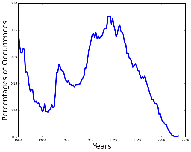
```
This shows the percentage of occurrences for the name Peter for the years 1880 to 2014.

Hints

The following are hints and suggestions that will help you complete this activity:

Use the str.split method to separate the comma-separated-values from the year files.
Remember that data read from a file is stored in a string. If you want a field to be another type (i.e. an int), then you must explicitly cast to that type.
Remember that the path to a file is simply a string, so you can use all your normal string methods such as str.format to build the path to a year file.
To compute the percentage, you can use the following formula:
```
percentage = count * 100.0 / total
```
Once you have your data organized, you can plot the graphs using the following code:
```
plt.figure(figsize=(10, 8))
plt.plot(years, occurrences, linewidth=4)
plt.xlabel('Years', fontsize=24)
plt.ylabel('Number of Occurrences', fontsize=24)
```
Play around with the parameters to figure, plot, xlabel, ylabel to stylize the plot to your liking.

Don't Print Large Files

If you try to print a large file you will most likely lock up your Notebook.

Questions

After completing the activity above, answer the following questions:

Described how you processed the data. What did you need to keep track of during your processing of the data? How was this information used to produce your plots? What difficulties did you encountered in processing the data and how did you overcome them?
Do the results of the plots surprise you? Where are there spikes in your graphs and what historical events would explain those spikes?

Activity 2: State Baby Names

For this activity, you are to do basically the same thing as in the previous activity, except on the state dataset (the national dataset was for all names in the nation, while this dataset is broken down by state).

Functions

To complete this activity, we can break the activity down into the following functions:

Count the yearly occurrences in a state file

def count_yearly_occurrences_in_state(path, baby_name):
    ''' Return a dict with the number of occurrences for the baby_name in each year '''

Given the path to a state file and a target baby_name, return a dict with the number of occurrences of the target baby_name in each year.

Once you have completed this function, you should be able to do the following:

>>> count_yearly_occurrences_in_state('state_baby_names/CA.TXT', 'Peter')
{1910: 12,
 1911: 18,
 1912: 47,
 1913: 47,
 ... SNIP ...
 2011: 241,
 2012: 221,
 2013: 237,
 2014: 233}

This means that the name Peter was given to 12 babies in 1910 in the state of California, 18 babies in 1911, etc.

Count the total yearly occurrences in a state file

def count_yearly_totals_in_state(path):
    ''' Return a dict with the total number of occurrences in each year. '''

Given the path to a state file, return a dict with the total number of occurrences in each year.

Once you have completed this function, you should be able to do the following:

>>> count_yearly_totals_in_state('state_baby_names/CA.TXT')
{1910: 9164,
 1911: 9984,
 1912: 17944,
 1913: 22094,
 ... SNIP ...
 2011: 436857,
 2012: 438069,
 2013: 430088,
 2014: 436552}

This means that there were a total of 9164 babies born in 1910, 9984 in 1911, etc.

Plot the state occurrences
```
def plot_state_occurrences(data):
    ''' Plot the number of occurrences for the state data '''
```
Given data returned from count_yearly_occurrences_in_state, plot the number of occurrences for each year.

Once you have completed this function, you should be able to do the following:
```
>>> data = count_yearly_occurrences_in_state('state_baby_names/CA.TXT', 'Peter')
>>> plot_state_occurrences(data)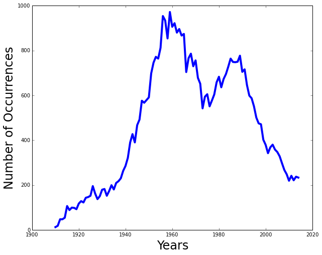
```
This shows the number of occurrences for the name Peter for the years 1910 to 2014 in California.
Plot the state percentages
```
def plot_state_percentages(data, totals):
    ''' Plot the percentages of occurrences for the state data '''
```
Given data returned from count_yearly_occurrences_in_state and the totals from count_yearly_totals_in_state, plot the percentage of occurrences for each year (i.e. number for that year / total for that year).

Once you have completed this function, you should be able to do the following:
```
>>> data   = count_yearly_occurrences_in_state('state_baby_names/CA.TXT', 'Peter')
>>> totals = count_yearly_totals_in_state('state_baby_names/CA.TXT')
>>> plot_state_percentages(data, totals)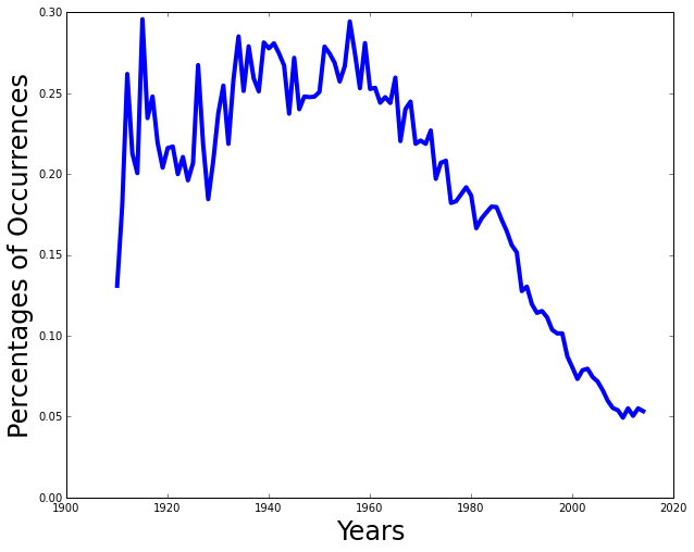
```
This shows the percentage of occurrences for the name Peter for the years 1910 to 2014 in California.

Hints

The following are hints and suggestions that will help you complete this activity:

Remember that a dict has a dict.get method where you can set a default value should a key not exist in the dict.
Remember that a dict provides access to a list of the key, value pairs via the dict.items method.
Remember that you can sort the items in dict using sorted.
You can implement count_yearly_totals_in_state in terms of count_yearly_occurrences_in_state if you interprete a None value for the baby_name parameter as matching any name.
To plot, you will need to separate the keys and values from the input data dict.

Questions

After completing the activity above, answer the following questions:

Described how you processed the data. Compare how you processed the data in this exercise with how you did it in the previous exercise. What was different? What was the same?
Do the trends for your birth state match the national trends? What reasons do you think would lead to these discrepancies if there are any?

Activity 3: Open Exploration

For the third activity, you are to produce two additional graphs or plots from the baby names dataset. Here is a list of some possible ideas, but you are more than welcome to come up with your own:

Plot the number of occurrences of two names on the same plot.
Plot the ratio of male to female names over time.
Create a histogram for a particular year or for particular name based on number of occurrences.
Plot the number of unisex names (that is names are used for both genders).
Compare the popularity of a name from multiple states on the same plot.
Compare your first and middle name on the same plot.
For each plot, write a summary that analyzes the data and what it means.

Hints

The following are hints and suggestions that will help you complete this activity:

As we have done in the previous activities, write smaller utility functions where each function has clear and focused purpose.
Re-use these smaller functions by combining them in another function to solve the overall problem.

Questions

For each plot or graph you produced, write a summary that describes how you collected the data for the figure, analyzes the results, and discusses the significance of the findings.

Submission

To submit your notebook, follow the same directions for Notebook00, except store this notebook in the notebook07 folder.