• Femtosecond Pump-Probe Spectroscopy
• Nanosecond Laser Flash Photolysis
• Electron Energy Loss Spectroscopy (EELS)
• Time-Correlated Single Photon Counting
• Diffuse Reflectance/Absorption Spectroscopy
• Fluorescent Upconversion
• Raman Spectroscopy
• Impedance Spectroscopy

Femtosecond transient absorption spectroscopy allows us to measure processes that occur on the picosecond timescale. Examples of these processes are: excited state energy transfer, inter- and intramolecular electron transfer reactions, charge transfer complexation and radical recombination in aqueous and nonaqueous solvents as well as in heterogeneous systems such as colloidal suspensions and thin films. We use the system mainly for measuring energy and electron transfer processes (both in colloidal suspensions and on thin films) in order to better understand how to construct photovoltaic devices. This spectroscopic method allows us to simultaneously record kinetic and spectral data regarding the excited state decay of our materials of interest.

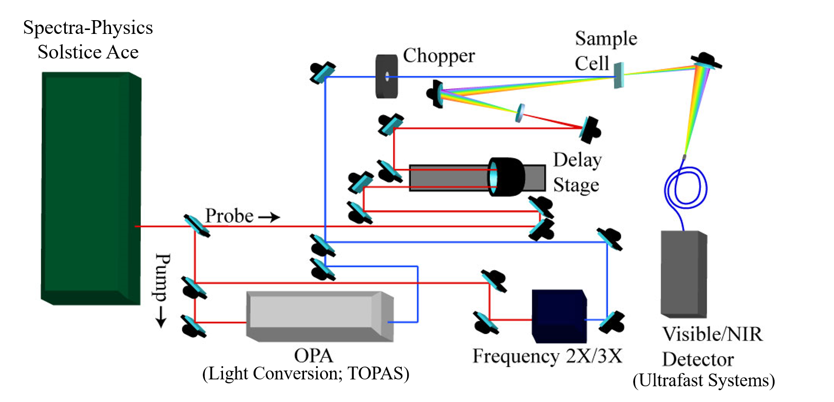
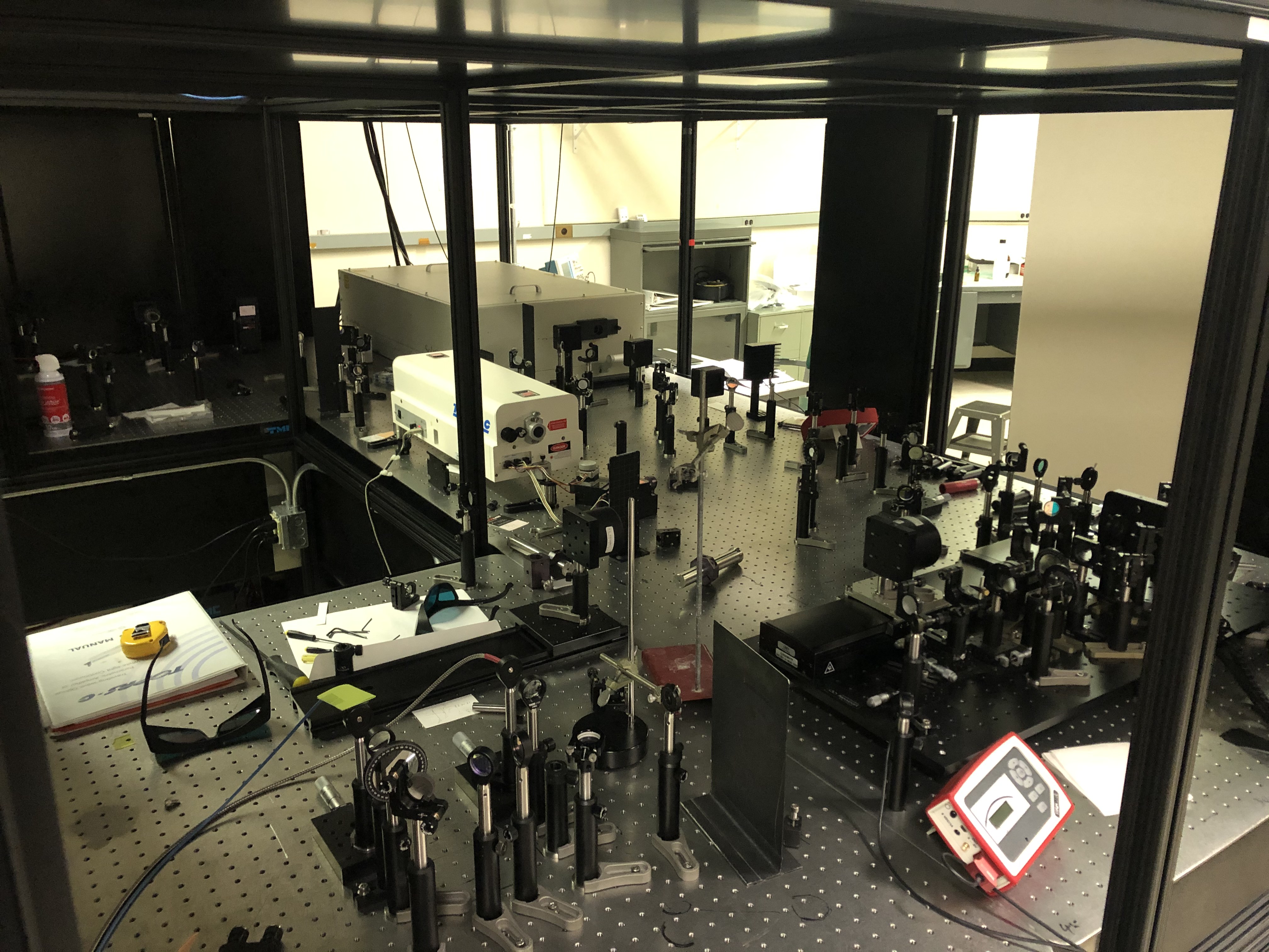
Figure. (Top) Schematic representation of the main components found in our femtosecond transient absorption system. In this system, pump and probe pulses measure the absorbance of a system in the ground state (Abs_probe) and after excitation by the pump (Abs_pump+probe) with subpicosecond time resolution. (Bottom) Photo of our set-up.

System Components
Our system (right) couples Helios software provided to us by Ultrafast systems with a Solstice-Ace laser from Spectra-Physics (800 nm fundamental, 1 kHz repetition rate) . In short, the fundamental is split 95/5 (pump/probe) and the 800 nm fundamental is frequency-doubled in a BBO crystal to generate 400 nm pump pulses. Alternatively, we can send the fundamental into an Optical Parametric Amplifier (OPA; LightConversion TOPAS) to generate pump wavelengths between 230-1600 nm.

Two key components of the system are the chopper and the delay stage. The chopper is used to remove a number of pump pulses from the pulse train at a certain frequency, allowing us to probe the sample in both the excited (Abs_pump+probe) and ground (Abs_probe) state. The resultant data collected is the difference between the two measurements (equation below).

ΔAbs = Abs(Pump + probe) – Abs(Probe)

The probe (5% of the 800 nm fundamental) is redirected through the delay stage, giving us the ability to stagger (in time) the arrival of the pump and probe pulses at the analyte. The pulse train is then sent through a Sapphire crystal in order to generate a white-light continuum (440-750 nm) and allow us the ability to make measurements over the majority of the visible spectrum. A near-IR continuum (900 -1500 nm) can also be generated for measurements in the NIR region. We have two spectrometers available for detection of probe wavelengths. The visible detector ranges from 200-1000 nm and the NIR detector from 800-1600 nm.

Measurement Limits
The laser pulse width (~30 fs) is an important factor in the measurement of kinetic data. Any process that occurs on roughly the same time-scale as the pulse width will be difficult to resolve kinetically, as its excited state dynamics will be obscured within the duration of the laser pulse.

The delay stage can accurately move a small enough distance to delay the pump and probe pulses by 20 fs (a delay stage translation of about 5 mm). The result of this is that we cannot accurately take data points less than 20 fs apart. The length of the delay stage is also a limiting factor in the system. The delay stage (0.48 m) only allows a total delay time of 1600 ps between pump and probe arrival time. With a longer delay stage we could take measurements over a larger time window however in most cases, a long delay stage can complicate the system setup causing the system to become impractical.

Nanosecond Laser Systems

Laser flash photolysis is a common method of probing photochemical reactions. A short pulse of laser light of a frequency which sample molecules absorb can promote large numbers of those molecules into excited states, from which they can fluoresce, react, or dissipate the excitation as heat. The growth and decay of concentrations of molecular species can be observed by optical absorption spectroscopy, diffuse reflectance spectroscopy, resonance Raman spectroscopy, fluorescence yields, microwave conductivity, or electron paramagnetic resonance spectroscopy. The characteristics of a number of lasers used for these purposes are described below.

Laser Cluster for Time-Resolved Photochemistry

• Nitrogen laser (337 nm / 6 ns)
• kinetic absorption spectroscopy
• fluorescence lifetimes
• 2-pulse experiments
• Excimer laser (308 nm / 20 ns)
• kinetic absorption spectroscopy
• 2-pulse experiments
• YAG laser (266, 355, & 532 nm / 6 ns)
• kinetic absorption spectroscopy
• fluorescence lifetimes
• microwave conductivity
• diffuse reflectance
• 2-pulse experiments

Laser Cluster for Inorganic Photochemistry

• Excimer laser (248 & 351 nm / 20 ns)
• kinetic absorption spectroscopy
• magnetic field effects
• 2-pulse experiments
• YAG laser (266, 355, & 532 nm / 6 ns)
• magnetic circular dichroism
• 2-pulse experiments

Laser Cluster for Time-Resolved Resonance Raman

• Dye laser (pumped by 308 nm excimer laser / 20 ns)
• Nitrogen laser (337 nm / 6 ns) GONE?
• Excimer laser (308 nm / 20 ns)

Time-Resolved Electron Spin Resonance

• Excimer laser (308 nm / 20 ns)

Fluorescence Laboratory

• YAG laser (355 & 532 nm / 0.1 ns / 5 kHz)
• fluorescence lifetimes (single-photon counting)

EELS is a technique used in comination with transmission electron microscopy (TEM). In EELS, a material is exposed to a beam of electrons with a known, narrow range of kinetic energies. As some of these electrons undergo inelastic scattering, lose energy and have their paths slightly and randomly deflected through interactions with the atoms in the sample, the amount of energy loss can be measured via an electron spectrometer. The amount of energy lost via inelastic scattering is directly related to specific inelastic interaction undergone, such as phonon excitations, inter and intra band transitions, plasmon excitations, inner shell ionizations, and Čerenkov radiation. This energy loss can therefore tell a significant amount about the energetic structure of the sample. Inner-shell ionizations are particularly useful for detecting the elemental components of a material since the electron energy loss of the incoming electron can be directly correlated with the energy level of the ionized electron. Within transmission EELS, the technique is further subdivided into valence EELS which measures plasmons and interband transitions, and inner-shell ionization EELS which can provide information on atomic composition from very small samples.

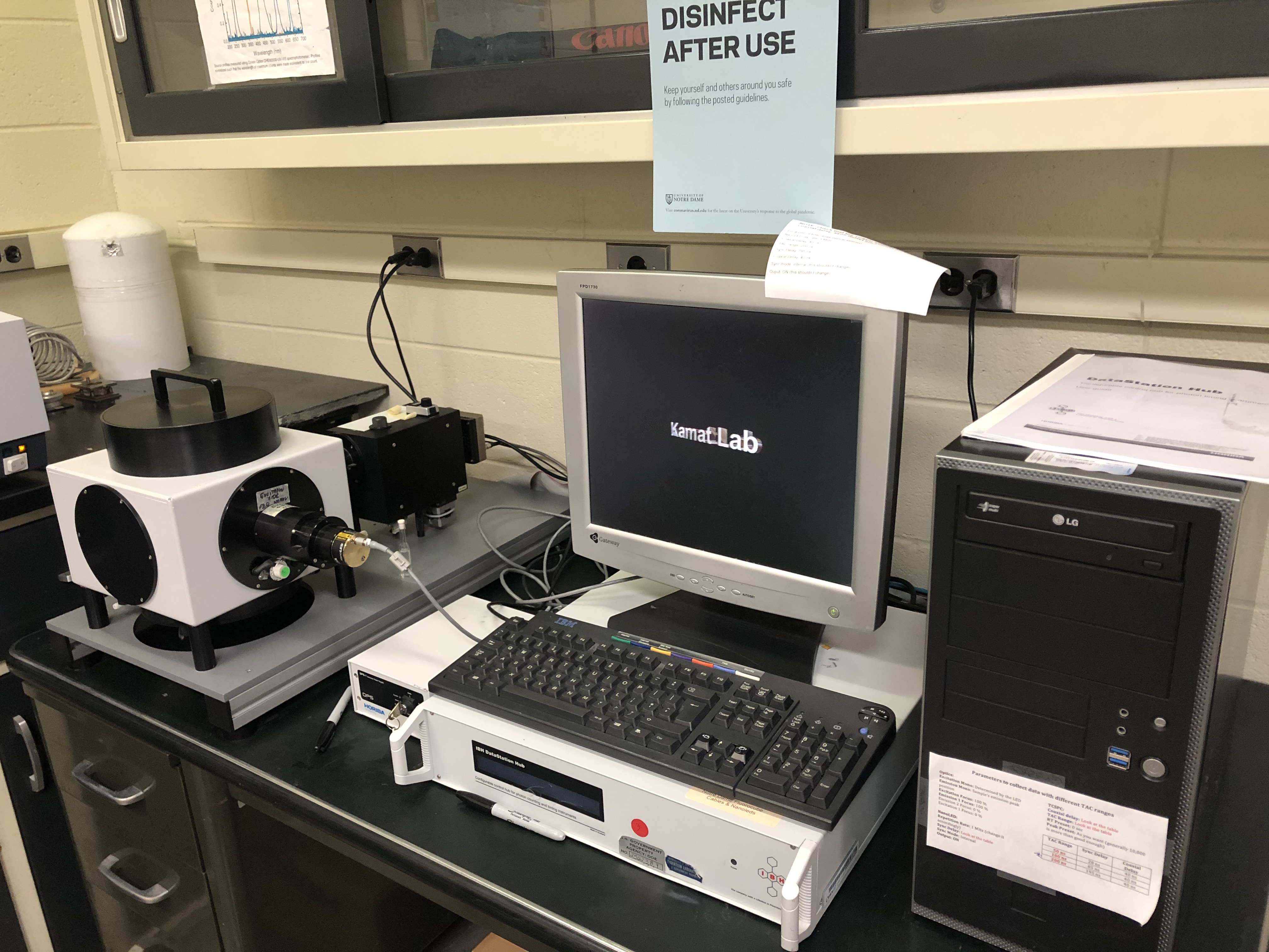
(Top) Schematic diagram of the components in the TCSPC system supplied by Horiba Scientific. (Bottom) Image of the table-top TCSPC system.

Time-Correlated Single Photon Counting (TCSPC or sometimes referred to as Emission lifetime) allows us to monitor emissive transitions in our materials (usually semiconductors or dyes) of interest. Characterizing emission in a time correlated fashion allows us to observe and characterize energy and electron transfer processes. Using TCSPC in combination with steady-state fluorescence we can calculate radiative (k_r) and nonradiative (k_nr) recombination rates for our materials of interest. From excited state lifetime data we can study systems that influence electron and energy transfer as well as make general observations about electron-hole separation in a material. These observations help to understand the best way modify materials (chemically, structurally etc…) so that they are more suitable for light conversion in a photovoltaic device.

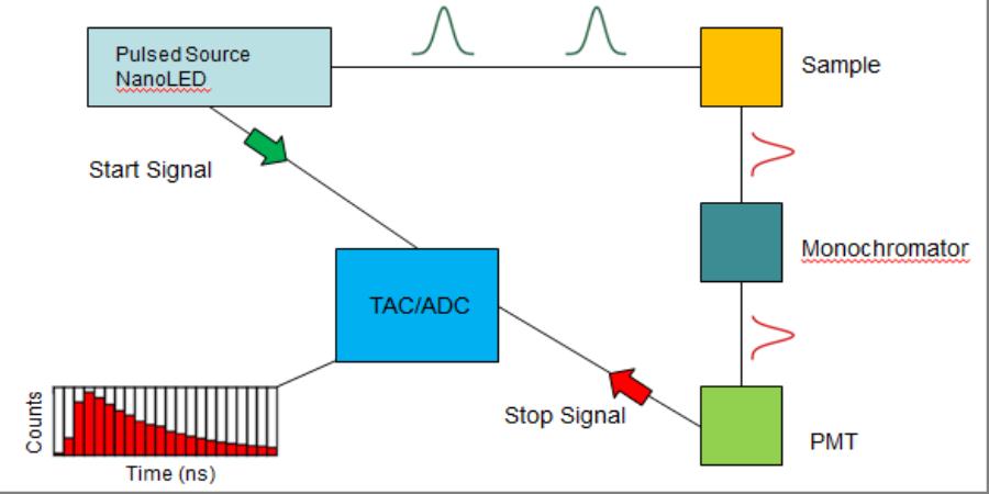
An experiment (the detection of a single photon) begins with a NanoLED excitation source with a pulse width of approximately 1 ns. Below is a step-by-step explanation of how the system works, the figure above supplies a visual explanation:

1. The LED sends an excitation pulse at the analyte (for the sake of giving it a name, let's call it colloidal CdSe Quantum Dots suspended in toluene) and at the same time sends an electrical start signal to the time-to-amplitude-converter (TAC) which is responsible for analog-to-digital conversion (ADC) of the final signal (see step 5 for a clearer description of the TAC/ADC).
2. The QDs absorb the excitation pulse and after a short period of time a fraction of the QDs re-emit photons in the direction of the detector.
3. These photons pass through a monochromator which is a device that is responsible for selecting the photons emitted from the transition of interest in the QDs. In some cases there may be multiple emissive transitions or a broad emission band for different analytes so this photon selection step is extremely important. Note: It is also important to use the appropriate optical filters to aid in the selection of the correct photons. These filters should be placed between the sample and the monochromator.
4. The photons that pass through the monochromator are then detected by a photomultiplier tube (PMT). In short, a photon of light generates a free electron inside of the PMT. The electron is then multiplied to become many electrons which are received at the TAC/ADC as the stop signal for the experiment.
5. The TAC/ADC, which is essentially just a highly accurate stop-watch, begins building a voltage when it receives the start signal and stops building the voltage when it receives the stop signal from the PMT. The voltage built during the absorption, re-emission and detection processes is the correlated to a time and plotted as one count (one photon) at the correlated time that is recorded by the TAC/ADC.
6. Based on the repetition rate (up to 1 MHz), this photon counting is repeated many times per second generating a plot of the number of photons counted at each time interval.

The resolution of the instrument is related to the PMT. It is of high importance to have only the desired wavelength of detection collected at the PMT. A stray photon of undesired wavelength that makes it to the PMT will be counted as a photon of the desired wavelength. A PMT is insensitive to the energy of a photon and only knows whether it receives or doesn't receive a photon. The PMT is responsible for supplying the time-correlated data in this experiment which makes it the limiting factor in making measurements.

Watch Jeff DuBose's lecture on Time Correlated Single Photon Counting (TCSPC) for Photoluminescence Lifetime Measurements:

Diffuse Reflectance and Ultraviolet-Visible Absorption Spectrometry are some of the most fundamental ways to probe the excited state of a wide variety of species. Fundamentally, these two techniques involve splitting white light into the entire rainbow of colors with a device called a monochromator (much the same as a prism does). Then the sample is illuminated with one specific wavelength, or color, of light and the amount that transmitted through the sample (in UV-Vis absorption spectrometry) or reflected off of the sample (in Diffuse Reflectance) is measured.

These spectra allow the electronic transitions in a molecule or semiconductor to be explored because, when a molecule, or semiconductor, absorbs a photon, an electron is promoted from an occupied state to an unoccupied state. If there is no electronic transition of the same energy as the photon, it is not absorbed.

By observing the energies of light that are absorbed we can determine the energies of these possible transitions in the species. The concentrations of species can also be determined from Diffuse Reflectance and UV-Vis Absorption Spectrometry using the Kubelka-Munk function and the Beer-Lambert law respectively. These relationships allow for the simplistic tracking of reactions, determination of concentrations, and are used extensively in daily scientific study.

The fluorescence upconversion (Ultrafast Systems Halcyone) system allows for the resolution of fluorescence lifetimes on the order of 230-300 fs. It employs a Ti:Sapphire oscillator femtosecond laser (Coherent Chameleon) as the excitation source and source of "gate" pulses. By controlling the time when "gate" pulses reach a nonlinear optical crystal using a delay rail, we control when upconversion can occur. Upconversion is a mixing of gate and fluoresced photons that results in a sum frequency signal of higher energy photons. By controlling when upconversion can occur, we know when the sample fluoresced with accuracy that is limited only by width of the "gate" pulse.

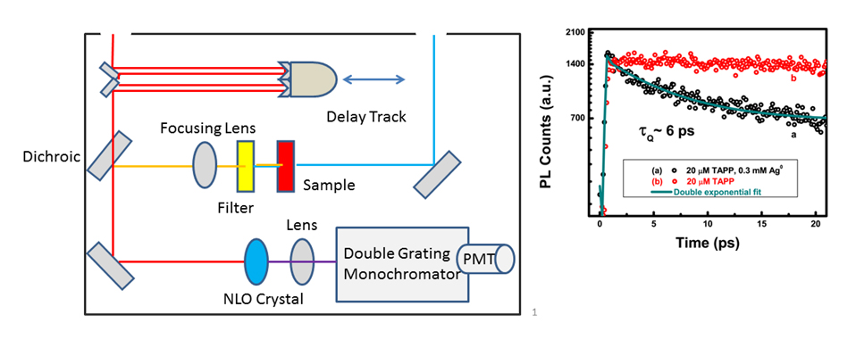
Fluorescence Upconversion Spectrometer and Data: Conceptual Schematic of the fluorescence upconversion spectrometer and example of fluorescence upconversion data for porphyrin and porphyrin-silver nanoparticle solutions. Plot reprinted with permission from {J. Phys. Chem. C, 2011, 115 (46) pp 22761 - 22769}. Copyright {2011} American Chemical Society).

Our group uses upconversion to measure fluorescence lifetimes of samples with very short-lived excited states. For example, for systems where we expect fast electron transfer from a donor to an acceptor, we can monitor quenching of the donor fluorescence which provides information about electron transfer kinetics. The high accuracy of upconversion measurements allows us to resolve fluorescence quenching kinetics that would not normally be observable by techniques such as Time-Correlated Single Photon Counting (TCSPC).

Figure: Schematic for process involved in collecting Raman spectra. The majority of scattered light is elastically scattered, meaning it is the same wavelength as the excitation source. A notch filter is used to block elastically scattered light which would otherwise overwhelm the weak signal from the Raman or inelastically scattered photons (~ 1/106 scattered photons1). The Raman scattered light may be dispersed according to wavelength and detected by a CCD. A Raman spectrum for tetra(4-aminophenyl) porphyrin (TAPP) powder is shown (Plot reprinted with permission from {J. Phys. Chem. C, 2011, 115 (46) pp 22761 - 22769}. Copyright {2011} American Chemical Society).

The microscope is often employed for surface enhanced Raman spectroscopy (SERS) which provides information about interaction between Raman active molecules and SERS active materials. Charge transfer interactions are indicated by an increase in the SERS signal. SERS greatly increases the sensitivity of a Raman measurement and allows for detection of trace amounts of chemical species.

Raman is a vibrational spectroscopy that provides rich information about the identity of molecular species (See Figure below). Our Raman instrument is a Renishaw Raman microscope (RM 1000) with two excitation sources: a 514 nm Argon ion laser and a 785 nm laser. The microscope is also equipped with a Prior ProScan III scanning stage for Raman mapping experiments. We are able to examine solution as well as solid samples using the microscope.

Halvorson, R. A.; Vikesland, P. J., Surface-Enhanced Raman Spectroscopy (SERS) for Environmental Analyses. Environmental Science & Technology 2010, 44 (20), 7749-7755.

Entry Here...